What Is a Market Correction? A Complete Investor’s Guide
Understand the 10% threshold, drawdown calculations and recovery math—and what a decline can and cannot tell you about investment risk.
A market correction is a decline of at least 10% from a relevant recent high. Financial markets rarely move in straight lines. Even during extended periods of economic expansion, rising corporate earnings, and strong investor confidence, stock prices can decline sharply. Sometimes these declines last only a few trading sessions. On other occasions, markets experience sustained selling pressure that erases months or even years of gains. One of the most important concepts investors encounter during these periods is the market correction.
A market correction is generally defined as a decline of at least 10% from a recent market high. When investors discuss a correction in the S&P 500, they are usually referring to a decline in the index’s price level from its previous peak. The definition is relatively simple. Its implications are considerably more complex. A correction can develop because investors reassess economic growth, interest rates, corporate profitability, geopolitical risks, or the prices they are willing to pay for future earnings. It can occur during an otherwise healthy economy, precede a recession, or emerge as part of a larger bear market.
The central challenge is that investors cannot reliably determine which outcome they are experiencing while events are unfolding. A 12% decline might eventually prove to be a temporary interruption in a long-term advance. Alternatively, that same decline might be the early stage of a much deeper downturn. Understanding market corrections therefore requires more than memorizing a percentage threshold. Investors need to understand how declines are measured, why markets reprice assets, how volatility interacts with long-term investment returns, and how individual financial circumstances influence the decisions that make sense during uncertain periods.
This guide explores those questions through financial analysis, mathematical examples, historical context, and practical investment principles. Start with the drawdown calculator or recovery calculator to test a hypothetical decline.
What Is a Market Correction?
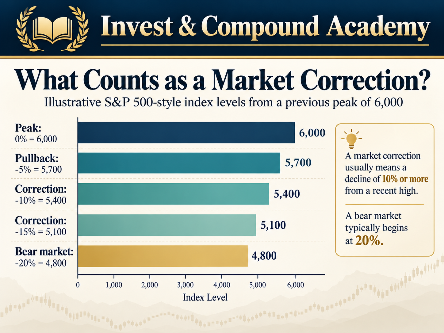
A market correction occurs when the price of a financial asset, market index, or broader market falls at least 10% below a relevant recent peak. The term is most frequently associated with major stock market indexes such as the S&P 500, Nasdaq Composite, and Dow Jones Industrial Average. However, the concept can also describe declines in individual stocks, industry sectors, commodities, and other assets. For example, imagine that the S&P 500 reaches an index level of 6,000. Several weeks later, the index falls to 5,400. The decline is 600 index points, representing 10% of the previous high.
At that point, the index has entered correction territory under the conventional definition. A subsequent decline to 5,100 would represent a cumulative loss of 15% from the original peak, not an additional correction measured independently from 5,400. This distinction is important because financial markets often experience temporary rallies during broader declines. A short-term rebound does not necessarily end the underlying drawdown or restore the previous market peak.
Understanding the Different Levels of Market Declines
Financial commentary uses several terms to describe downward price movements.
| Market condition | Commonly used definition |
|---|---|
| Minor decline | A relatively small decline, generally below 5% |
| Pullback | Often a decline of approximately 5% to less than 10% |
| Market correction | A decline of at least 10% but less than 20% |
| Bear market | A decline of 20% or more |
| Market crash | A particularly sudden and severe decline, without one universally accepted numerical threshold |
These categories are conventions rather than formal economic laws. Different researchers may use closing prices, intraday values, adjusted data, or different rules for identifying market peaks and subsequent recovery periods. Consequently, two legitimate studies can report somewhat different numbers of historical corrections. The 10% threshold should be understood as a useful classification boundary, not evidence that financial markets undergo a fundamental transformation the moment an index reaches that percentage. A market that is down 9.8% may face almost the same underlying economic conditions as one that is down 10.2%.
What matters is the combination of underlying causes, portfolio exposure, liquidity needs, valuations, and the investor’s ability to withstand further losses.
How Is a Market Correction Calculated?
The conventional calculation compares the current price or index level with a previous peak.
Suppose an index reaches 5,500 before declining to 4,840. The calculation is:
The market has experienced a 12% drawdown from its previous high. An investor who held an index-tracking investment throughout that decline would experience a similar percentage loss before fund expenses, distributions, tracking differences, and other portfolio-specific factors.
Price Decline Versus Dollar Loss
The percentage decline of an index does not automatically tell investors how much money they have lost. Consider three portfolios that experience the same 12% decline.
| Starting investment | Decline | Remaining value | Unrealized loss |
|---|---|---|---|
| $10,000 | 12% | $8,800 | $1,200 |
| $50,000 | 12% | $44,000 | $6,000 |
| $250,000 | 12% | $220,000 | $30,000 |
The market performance is identical in percentage terms, but its financial and emotional significance can differ substantially. A younger investor with decades until retirement may have the flexibility to endure volatility without changing planned withdrawals. Someone who needs to use their portfolio to purchase a home within six months may face a materially different problem. For that investor, a 12% decline could force the liquidation of investments at an unfavorable time. This illustrates an important principle: market risk is not determined solely by how far asset prices can fall. It is also determined by when an investor may need access to capital.
Maximum Drawdown
Analysts use the term maximum drawdown to describe the largest peak-to-trough decline within a specified observation period. Suppose a portfolio follows this sequence:
- January: $100,000
- February: $108,000
- March: $103,000
- April: $94,000
- May: $90,000
- June: $96,000
The relevant peak is $108,000, and the subsequent trough is $90,000. The drawdown is:
An investor who measures the decline only against the original January value would conclude that the portfolio is down 10%. That figure may describe the change since January, but it does not accurately describe the maximum drawdown from the highest preceding value. This distinction matters when comparing investment strategies, ETFs, managed portfolios, and historical market downturns. An investment may generate an attractive long-term return while still exposing investors to substantial interim drawdowns.
Market Correction Drawdown Calculator
Use a peak and current level from the same price series. The dollar illustration assumes the entered amount was invested at the peak, without cash flows or other costs.
The category uses the unrounded decline. It is a conventional label, not a signal to buy or sell. A current quotation alone cannot establish an episode’s eventual trough or recovery date.
Why Do Market Corrections Happen?
Understanding an earnings-driven decline starts with the business itself. Our guide to reading a stock’s key financial numbers explains how profitability, valuation and debt fit into that assessment.
Market corrections rarely have a single isolated cause. Financial markets are forward-looking systems in which investors continuously update expectations about future earnings, economic conditions, interest rates, and risk. The market price of a stock represents what buyers and sellers are willing to exchange for ownership at a particular moment. When investors collectively become less optimistic about the future, market prices can fall even if companies remain profitable and current economic data appear reasonably healthy.
Changes in Interest Rates
Interest rates influence the valuation of financial assets. A simplified valuation model estimates the present value of future cash flows by discounting those cash flows at a rate that reflects the time value of money and investment risk. When required returns rise, the present value of future cash flows generally falls, all else being equal. For example, consider a company expected to generate $100 in cash flow for shareholders five years from now. Using an illustrative discount rate of 6%, the present value of that cash flow is approximately $74.73. If the required discount rate increases to 9%, its present value falls to approximately $64.99.
The expected future payment has not changed. Only the rate used to value that payment has increased. This is one reason growth-oriented companies can be especially sensitive to changes in interest-rate expectations. A company whose valuation depends heavily on profits expected many years into the future may experience a larger revaluation than a mature business generating substantial current cash flow. However, interest rates do not affect every company or industry in exactly the same way. Banks, utilities, real estate businesses, technology companies, and highly leveraged corporations can respond differently depending on their business models, balance sheets, funding structures, and competitive environments.
Inflation and Monetary Policy
Inflation measures the rate at which the general price level of goods and services rises. Moderate inflation may coexist with economic expansion and corporate profit growth. Unexpectedly high or persistent inflation, however, can create additional uncertainty. Businesses may face rising labor costs, transportation expenses, financing costs, or raw-material prices. Some companies can pass those increases to customers without substantially reducing demand. Others cannot. At the same time, central banks may respond to inflation by raising policy interest rates or maintaining restrictive financial conditions. Higher borrowing costs can slow economic activity, reduce credit demand, and make financing more expensive.
The resulting combination of inflation uncertainty, tighter monetary policy, and weaker expectations for corporate earnings can contribute to falling equity valuations. Nevertheless, inflation does not automatically cause a market correction. Markets react to the difference between actual developments and expectations already incorporated into prices. An inflation report that appears high in absolute terms may be received positively if investors expected an even worse result.
Corporate Earnings Disappointments
Stock prices reflect expectations about company profits, cash generation, and future growth. A business may report record revenue and still experience a sharp share-price decline. Financial markets evaluate results relative to expectations. If investors have already priced in extremely strong earnings growth, even an impressive report can disappoint. Consider a fictional company trading at $150 per share with expected annual earnings of $5 per share. Its forward price-to-earnings ratio is 30. Suppose earnings expectations decline to $4.50 and investors become willing to pay only 25 times forward earnings. The implied share price becomes:
That represents a 25% decline from $150. The decline reflects two forces operating together: lower expected earnings and a lower valuation multiple. Across a broad index, the same mechanism can produce a correction when investors collectively lower profit expectations or reduce the multiples they are prepared to pay.
Economic Growth Concerns
Stock markets often decline before a recession becomes evident in official economic statistics. Investors may observe signs of weakening consumer spending, slower industrial production, rising unemployment, reduced capital investment, or deteriorating lending conditions. They may begin selling equities because they expect future earnings to weaken. However, the relationship between economic conditions and financial markets is not perfectly predictable. Markets sometimes recover before a recession ends. They can also experience corrections without a recession occurring at all. The stock market and the economy are connected, but they measure different things.
Economic statistics describe production, employment, spending, and other real-world activity. Equity prices reflect investor expectations concerning future business outcomes. Because expectations change continuously, the market frequently moves ahead of published economic data.
Geopolitical Developments
Wars, trade disputes, political instability, supply-chain interruptions, and unexpected changes in government policy can affect markets. The financial consequences depend on how events influence energy prices, trade flows, business confidence, inflation, financing conditions, and corporate earnings. An interruption in a critical shipping route, for example, could raise transportation costs and reduce the reliability of supply chains. Companies dependent on imported components may experience production delays. Investors may respond by reassessing profits and demanding a larger risk premium. Nevertheless, the direction and duration of the market response remain uncertain.
Financial markets sometimes absorb geopolitical shocks surprisingly quickly when the direct economic consequences prove smaller than initially feared. At other times, apparently contained events develop into broader disruptions.
Investor Sentiment and Positioning
Market prices are influenced not only by economic fundamentals but also by behavior. During prolonged periods of rising prices, optimism can become increasingly widespread. Investors may extrapolate recent returns into the future, assume valuations will continue expanding, or underestimate the possibility of losses. When market sentiment changes, those expectations can reverse. A decline may trigger further selling as investors reduce risk, close leveraged positions, or react to negative headlines. This process can temporarily push prices away from levels justified by long-term business fundamentals. However, a decline driven partly by sentiment is not necessarily irrational.
Sentiment and fundamentals interact, and investors often have difficulty determining how much of a price change reflects genuine economic deterioration.
How Market Corrections Develop
A correction does not follow a predetermined sequence. Nevertheless, certain patterns appear repeatedly in financial market history.
The Initial Reassessment
A market advance may begin slowing after valuations rise, earnings expectations become demanding, or economic conditions become less supportive. The first stage can be subtle. Major indexes may continue approaching record highs even as fewer companies participate in the advance. Some industries weaken while others continue rising. Investors may initially regard these developments as ordinary fluctuations rather than evidence of a broader shift.
The First Significant Decline
A disappointing economic report, earnings announcement, policy development, or unexpected event may trigger more substantial selling. Volatility increases as market participants reassess risk. At this point, some investors purchase shares because they believe the lower price represents an opportunity. Others reduce exposure because they expect conditions to deteriorate. Both groups are responding to uncertainty, but they are operating under different assumptions about the future.
The Expansion of Selling Pressure
As the decline develops, more companies or market sectors may participate. Investors who initially ignored the weakness may begin reconsidering their positions. Stop-loss orders, margin requirements, fund redemptions, and derivatives-related hedging can amplify price movements. A market that initially appeared resilient may experience several unusually volatile trading sessions. Importantly, this does not mean markets always decline continuously. Short-term rallies can occur throughout a correction. A market may rise strongly for several days and subsequently fall to a new low.
Stabilization and Price Discovery
Eventually, selling pressure may diminish. Lower valuations can attract investors who judge the prospective return more favorably. Economic information may improve, policy uncertainty may decrease, or corporate results may exceed reduced expectations. The market may begin stabilizing. Yet investors cannot know in real time whether the lowest price has been reached. A temporary recovery may develop into a sustained advance or be followed by another decline. This uncertainty is one of the defining difficulties of investing through corrections.
Market Correction vs. Bear Market
The most widely recognized distinction concerns the size of the decline. A correction is conventionally associated with a decline between 10% and less than 20%. A bear market begins when the decline reaches at least 20% from a relevant peak. For example, suppose the S&P 500 reaches 6,000. At 5,400, the index is down 10%. At 5,100, it is down 15%. At 4,800, it is down 20%. The final level crosses the conventional bear-market threshold. However, a correction does not have to become a bear market. A market can decline 12%, stabilize, and eventually recover without ever experiencing a 20% peak-to-trough loss.
Conversely, a bear-market decline crosses the 10% threshold on its way to a loss of 20% or more; a price gap can carry it through that range without trading at every intermediate level. The terminology also does not tell investors why prices are falling. A sharp decline associated with temporarily elevated interest-rate expectations differs from a prolonged downturn caused by deteriorating corporate profitability and severe credit-market stress. The comparison here establishes the definitions; a detailed comparison of correction and bear-market behavior is a separate research question.
How Long Do Market Corrections Last?
There is no predetermined duration. A correction may reach its lowest level in a matter of days or extend across several months. Recovery to a previous high can take considerably longer than the decline itself. It is therefore essential to distinguish between two different measurements. Peak-to-trough duration measures how long the market takes to decline from its previous peak to the eventual low. Full recovery duration measures how long it takes to regain the previous peak after the decline begins. These periods should not be treated as interchangeable.
A market that falls 15% over two months and then takes another eight months to regain its previous high experienced a two-month peak-to-trough decline but a ten-month peak-to-recovery period. Some historical studies report the former; others emphasize the latter. Fidelity’s historical research has documented substantial variation in both correction severity and duration, depending on the observation period and the criteria used. For example, an older Fidelity study covering S&P 500 correction episodes through June 2010 reported a median correction magnitude of approximately 12% and a median peak-to-trough duration of 54 days under its methodology.
Those figures are useful historical context, but they should not be interpreted as predictions of the next correction. See the historical report, page 25, for its sample and methodology. A more recent or differently constructed sample may produce different averages.
Why Historical Averages Have Limitations
Imagine five hypothetical corrections lasting 15, 35, 50, 80, and 220 days. Their average duration is 80 days. Their median duration is only 50 days. The unusually long episode meaningfully influences the average. Financial market observations also are not independent repetitions of the same experiment. Economic policy, market structure, investor behavior, valuation levels, and the global financial system evolve over time. Historical statistics can describe what has happened, but they cannot establish exactly when a future recovery will occur.
How Often Do Market Corrections Occur?
Investors sometimes regard a 10% market decline as evidence that financial conditions have become exceptional. History suggests that meaningful interim declines have been a recurring feature of equity investing. According to Fidelity research updated in March 2026, the S&P 500 experienced an intrayear decline of at least 10% in 48% of calendar years from 1980 through 2025. Over that same observation period, the average calendar-year total return was positive.
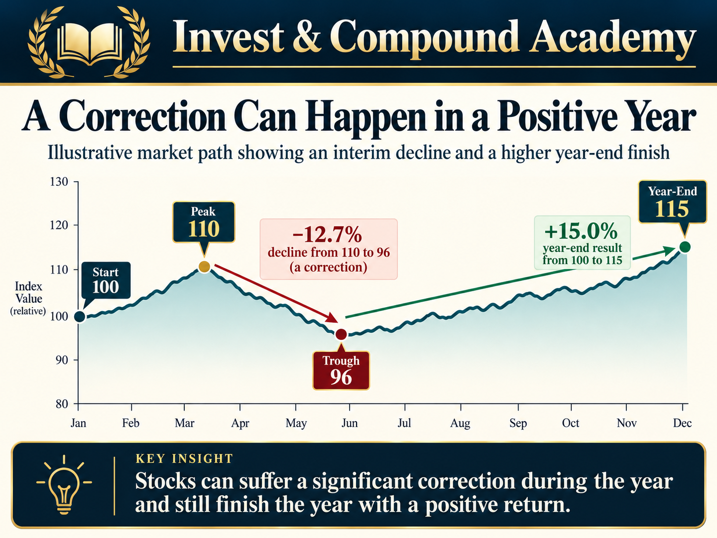
The Fidelity article identifies the data as ending December 31, 2025; 48% refers to calendar years with a qualifying intrayear drawdown, not the probability of a correction in the next year. These two findings are not contradictory. A stock market can experience a substantial temporary decline and still finish the calendar year with a gain.
Consider an illustrative index that begins a year at 100, rises to 110, declines to 96, and finishes at 115. The index experiences a peak-to-trough decline of approximately 12.7%, qualifying as a correction. Yet its full-year price return is positive 15%, before any dividends. An investor who observes only the annual starting and ending values would never see the magnitude of the temporary decline. This is why calendar-year returns alone provide an incomplete picture of investment risk. The illustrated annual result is a price return, while the Fidelity annual-return series cited above includes dividends.
Corrections Are Not Distributed Evenly
It would be misleading to interpret the historical frequency of corrections as a reliable calendar schedule. Markets do not automatically decline 10% after a certain number of months or years. Several corrections can occur close together. Other periods may feature extended advances without a significant decline. The frequency also varies according to the index being studied. A concentrated technology index can behave differently from a broad-market index. Small-cap stocks, international equities, and particular sectors may experience corrections at different times. An investor therefore should not assume that an index’s correction history can be applied directly to every individual security.
Historical Examples of Market Corrections
Historical episodes help illustrate the range of possible market outcomes. They also demonstrate why seemingly similar percentage declines can have very different underlying causes.
The 2010 European Debt-Crisis Period
In 2010, concerns about sovereign debt and financial stability in parts of Europe contributed to significant market uncertainty. Investors questioned whether fiscal pressures could disrupt banking systems, credit markets, and economic growth. U.S. equities experienced a substantial decline during the spring and early summer. Fidelity’s report measured a roughly 15% decline between April 23 and its June 30, 2010, reporting cutoff, using closing price-index data. That cutoff should not be mistaken for confirmation of the episode’s final trough. The episode illustrates how financial stress originating outside the United States can influence U.S. equity valuations.
It also demonstrates the importance of understanding the connection between sovereign debt, financial institutions, credit availability, and investor confidence.
The 2018 Market Declines
During 2018, financial markets confronted changing interest-rate expectations, inflation concerns, trade tensions, and uncertainty about the outlook for economic growth. The year included more than one period of significant market weakness. An early decline occurred as investors adjusted to the possibility of tighter monetary conditions. Later in the year, concerns surrounding trade policy, growth, and financial conditions contributed to another pronounced selloff. These episodes highlight an important feature of market risk: the same calendar year can contain different market corrections driven by a changing combination of economic and financial factors.
They also show why historical episodes should be measured carefully rather than reduced to a single headline.
The 2020 Pandemic Collapse
The onset of COVID-19 produced a rapid global market decline as investors confronted extraordinary uncertainty about economic activity and business operations. The S&P 500 fell far beyond the 10% correction threshold and entered bear-market territory. Travel restrictions, business shutdowns, deteriorating economic expectations, and financial-market stress contributed to the decline. Subsequent monetary and fiscal policy responses, changing expectations, and economic adaptation influenced the recovery. The episode demonstrates why investors cannot assume that a decline will stop at 10% or 15%. A correction threshold is a description of how far prices have already fallen, not a protective boundary.
The 2022 Inflation and Interest-Rate Environment
In 2022, rising inflation and a substantial shift toward tighter monetary policy contributed to pressure on equity valuations. Higher discount rates affected long-duration growth investments, while investors reconsidered economic growth and corporate profitability. The S&P 500 ultimately experienced a bear-market decline. For investors, the episode provides a useful illustration of how valuation risk can emerge even when many companies remain operationally sound. The market price of an investment depends not only on company quality but also on the price paid for its expected future cash flows.
The Broader Historical Lesson
These events involved different catalysts and unfolded under different economic conditions. Their common feature was the repricing of uncertainty. Investors who understood the difference between temporary volatility, changing fundamentals, and liquidity constraints were better positioned to evaluate their decisions rationally. Nevertheless, history provides no guarantee that a particular asset, sector, or portfolio will recover. Broad market indexes can replace weaker companies over time, while individual investments may suffer permanent losses.
Why a Market Correction Does Not Always Mean Stocks Are Cheap
One of the most common misunderstandings about corrections is the assumption that any asset declining by 10% has become inexpensive. A lower price does not necessarily represent attractive value. Suppose a company’s shares initially trade at $200, while estimated sustainable annual earnings are $5 per share. The price-to-earnings ratio is 40. The stock subsequently declines by 15%, reaching $170. If earnings expectations remain unchanged, its price-to-earnings ratio falls to 34. The shares are cheaper relative to their previous price. However, a valuation of 34 times earnings may still be demanding depending on the company’s growth prospects, financial condition, competitive advantages, and risk.
Now consider a second possibility. The stock declines to $170, but expected earnings fall from $5 to $4. Its forward P/E ratio becomes 42.5. Our P/E ratio guide explains why a lower share price need not mean a lower earnings multiple. Despite the 15% share-price decline, the stock has actually become more expensive relative to its revised earnings outlook. This example illustrates why price declines must be evaluated alongside fundamentals.
Relative Price and Intrinsic Value
Relative price describes how much an asset costs compared with a previous market quotation or another investment. Intrinsic value refers to an estimate of an asset’s economic worth based on its future cash flows, risk, and other fundamental characteristics. The two concepts can diverge. A company can experience a temporary share-price decline while its estimated intrinsic value remains relatively stable. Alternatively, deterioration in its business outlook can cause intrinsic value to fall faster than its market price. Investors who equate lower prices with better value may overlook the possibility of fundamental impairment.
A sound investment assessment therefore considers both the price being offered and what the underlying asset is reasonably expected to produce.
What Happens to ETFs During a Market Correction?
Distinguish the fund structure from the risk of its holdings. Our ETF vs Stock comparison explains how owning a basket differs from owning one company, while retaining exposure to broader market declines.
Exchange-traded funds provide exposure to baskets of securities, market indexes, sectors, bonds, and other investment strategies. Their performance during a correction depends primarily on the assets and strategies they hold. An ETF tracking the S&P 500 generally will experience market movements broadly consistent with the underlying index, subject to tracking differences, fees, distribution mechanics, and other factors. A technology-sector ETF may experience a larger decline when selling pressure is concentrated in growth-oriented companies. A short-duration government bond ETF may behave differently because its underlying securities have different risk characteristics. However, diversification within an ETF does not eliminate market risk.
An equity ETF holding hundreds of companies can still fall substantially when broad stock markets decline.
Market-Capitalization Weighting
The S&P 500 is a float-adjusted market-capitalization-weighted index. This means companies with larger publicly tradable market values generally exert greater influence over index performance. A decline concentrated among the largest companies can therefore have a substantial impact on the overall index. Conversely, many smaller constituents may decline without producing an equally large index-level correction if the largest companies remain strong. This is why investors sometimes examine market breadth alongside headline index performance. Market breadth evaluates how widely price advances or declines are distributed across individual securities. For a comparison of different equity exposures, see VOO vs QQQ. It can add context, although it is not a reliable standalone predictor of future market direction.
Price Return and Total Return
Investors should also distinguish between price returns and total returns. A price-return index reflects changes in prices without including the reinvestment of ordinary cash dividends. A total-return index incorporates the effect of reinvested distributions according to the index provider’s methodology. The difference can become significant over long periods. Historical correction studies often use price-index levels, while long-term investment growth comparisons frequently use total-return data. Comparing these figures without understanding their definitions can lead to inaccurate conclusions. Our Dividend Yield vs Total Return guide separates distributions from overall performance. For background, use our guides to ETF foundations, ETF research and how the S&P 500 works.
The Mathematics of Recovering From a Correction
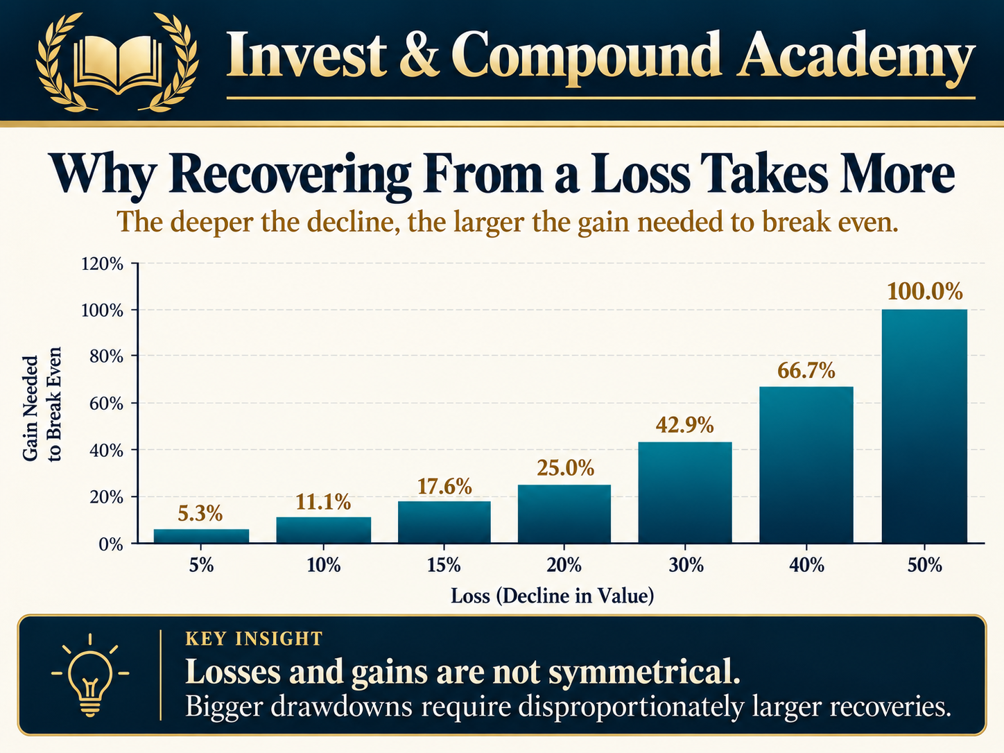
Investment losses and subsequent recoveries are mathematically asymmetric. A portfolio that declines 10% must gain more than 10% to return to its original value. Suppose an investment begins at $10,000. After a 10% decline, its value is $9,000. To recover the $1,000 loss, the investment must increase by:
The required recovery percentage grows as losses deepen.
| Portfolio decline | Remaining value from $10,000 | Required gain to recover |
|---|---|---|
| 5% | $9,500 | 5.26% |
| 10% | $9,000 | 11.11% |
| 15% | $8,500 | 17.65% |
| 20% | $8,000 | 25.00% |
| 30% | $7,000 | 42.86% |
| 40% | $6,000 | 66.67% |
| 50% | $5,000 | 100.00% |
This mathematical relationship is fundamental to risk management. As losses deepen, the proportional gain required for recovery increases at an accelerating rate. A portfolio that loses half its value must double to return to its previous level. However, this does not mean investors can automatically improve long-term performance by attempting to avoid every decline. Selling before a correction requires making a sufficiently accurate judgment about future losses. Reentering the market requires another decision about future gains. Both decisions involve uncertainty, transaction costs, potential taxes, and the possibility of missing a rapid recovery.
Understanding recovery mathematics is useful for evaluating risk, but it does not establish that active market timing will outperform a disciplined long-term strategy.
Loss Recovery Calculator
Compare the loss with the gain needed to regain the starting nominal value. No deposits, withdrawals, distributions, fees or taxes are included.
Required gain = decline ÷ (1 − decline), with the decline expressed as a decimal. At a 100% loss, no finite percentage gain on the zero balance can restore the starting amount. The calculation does not predict whether a recovery occurs.
How Market Corrections Affect Different Investors
Two investors can own the same ETF and experience the same market decline but face completely different financial consequences. The difference lies in their investment objectives, time horizons, income needs, liquidity, and financial resilience.
The Long-Term Accumulation Investor
An investor contributing regularly toward a retirement goal several decades away may be able to tolerate temporary declines. If income remains stable and emergency savings are adequate, the investor may continue making scheduled contributions. During a correction, the same contribution can purchase more ETF shares than it could at the previous higher price. Whether those purchases ultimately generate attractive returns depends on future performance. Lower prices increase the number of shares purchased for a fixed contribution, but they do not eliminate the possibility of further losses.
The Investor Approaching Retirement
An investor planning to retire soon may face greater sensitivity to portfolio declines. Even if the portfolio eventually recovers, withdrawals made during the downturn can reduce the capital available to participate in that recovery. This introduces sequence-of-returns risk. For example, two retirees may achieve the same average annual investment return over a long period but experience different portfolio outcomes because their positive and negative returns occur in different sequences while withdrawals are being made. Early losses combined with withdrawals can be particularly damaging.
A retirement strategy therefore needs to account for spending requirements, cash reserves, asset allocation, withdrawal flexibility, and the possibility of prolonged market weakness.
The Short-Term Investor
Someone saving for a near-term obligation generally has a different risk profile. Consider an investor who expects to make a $40,000 home down payment in eight months. If the full amount is invested in equities and falls by 15%, the portfolio would decline to $34,000. The investor may not have enough time to recover before the payment becomes due. For objectives with relatively inflexible dates, the capacity to tolerate market losses may be limited regardless of the investor’s emotional willingness to accept volatility.
The Leveraged Investor
Leverage introduces additional risk. An investor borrowing money to purchase securities may face margin requirements that become more demanding as market values fall. Declining collateral values can trigger requests for additional funds or forced liquidation. This means leveraged investors may be unable to hold through a correction even if they believe prices will eventually recover. The combination of falling markets, financing costs, and forced sales can create losses far larger than those associated with an unleveraged investment. For this reason, leverage should not be evaluated solely in terms of its potential to increase returns.
Its effect on liquidity, downside exposure, and the investor’s ability to control the timing of transactions is equally important.
Investor Psychology During a Market Correction
Market corrections are not simply financial events. They are also psychological tests. When asset prices decline, investors experience uncertainty about whether losses will deepen, how long recovery may take, and whether their original investment assumptions remain valid. Behavioral finance identifies several mechanisms that can influence decisions during these periods.
Loss Aversion
Loss aversion describes the tendency for losses to feel more significant than equivalent gains. An investor may experience considerable distress after losing $5,000 even though a previous $5,000 gain produced less satisfaction. This emotional asymmetry can encourage impulsive selling. The problem is not that concern about losses is irrational. Financial losses can have real consequences. The difficulty arises when the emotional discomfort of a temporary decline leads investors to abandon a strategy without evaluating whether their financial objectives or underlying investment assumptions have changed.
Recency Bias
Recency bias occurs when recent events receive disproportionate influence in expectations about the future. During a prolonged bull market, investors may begin assuming positive returns are normal and that substantial losses are unlikely. During a correction, several consecutive negative trading sessions can create the opposite impression. Investors may begin expecting prices to continue falling indefinitely. Neither expectation necessarily reflects a balanced assessment of longer-term possibilities.
Herd Behavior
Investors often observe what others are doing before making decisions. During periods of uncertainty, a high volume of selling can create the impression that other market participants possess superior information. However, observed trading activity does not reveal the objectives or constraints behind every transaction. One investor may be selling because of a margin call. Another may be rebalancing a portfolio. A third may be raising cash to meet an immediate obligation. A fourth may be expressing a negative outlook on future earnings. Treating all selling activity as evidence of the same economic conclusion can lead to mistaken interpretations.
Confirmation Bias
Confirmation bias involves placing disproportionate weight on information that supports an existing belief. An investor expecting a major crash may focus exclusively on negative economic forecasts. An investor convinced that markets will quickly recover may disregard legitimate signs of deteriorating fundamentals. Both behaviors weaken analytical discipline. A more effective process involves identifying the evidence that could invalidate an investment thesis. For example, an investor who believes a company is attractively valued might examine whether expected cash flows, competitive positioning, or debt obligations could deteriorate under a less favorable scenario. The objective is not to eliminate uncertainty but to evaluate it systematically.
Should Investors Sell During a Market Correction?
There is no universally correct answer. Selling during a correction can be reasonable under certain circumstances, but selling solely because prices have declined may also create avoidable long-term consequences. The relevant question is whether the investment continues to fit the investor’s objectives and financial circumstances.
When Selling May Be Justified
A decision to reduce exposure may be consistent with a sound financial plan when an investor’s liquidity needs have changed, a position has become excessively concentrated, leverage creates unacceptable risk, or the original investment thesis has deteriorated. For example, suppose a portfolio was intended to contain 60% equities and 40% fixed-income investments, but subsequent investment decisions increased equity exposure to 90%. A correction may expose the mismatch between the actual portfolio and the investor’s risk tolerance. Reducing exposure could be appropriate, although the timing and method deserve careful consideration.
Similarly, selling a company after discovering that its debt obligations are unsustainable may reflect fundamental risk management rather than emotional market timing.
When Selling May Be Counterproductive
An investor with a diversified portfolio, adequate cash reserves, stable income, and a long investment horizon may not need to change strategy simply because the market is down 12%. Selling creates a new decision: when to buy back. If prices recover rapidly, remaining in cash can mean missing part of the rebound. Investors should therefore distinguish between reacting to changing fundamentals and reacting to short-term discomfort. The presence of losses alone does not establish that an investment strategy has failed.
Should Investors Buy During a Market Correction?
Buying during a correction can offer access to assets at lower prices. However, lower entry prices do not guarantee positive future returns. An investor purchasing an ETF after a 10% decline may experience an additional 10%, 20%, or larger loss before prices recover. Buying should therefore be evaluated within an established allocation and risk-management framework.
An Illustrative Example
Assume an ETF trades at $100 per share before declining to $88. An investor contributing $1,000 could purchase approximately 11.36 shares at the lower price, assuming fractional shares are permitted and ignoring costs. At $100 per share, the same contribution would purchase 10 shares. The decline increases the number of shares obtainable for the same contribution. If the ETF later returns to $100, the shares purchased at $88 would have appreciated by approximately 13.64%, excluding distributions and expenses. However, if the ETF declines further to $70, that purchase would have an unrealized loss of approximately 20.45%. The example demonstrates both sides of the opportunity.
A correction can improve the prospective return from an unchanged future cash-flow stream, but it also may reflect genuine deterioration in expected returns, earnings, or risk.
Dollar-Cost Averaging
Dollar-cost averaging involves investing a fixed amount at regular intervals rather than attempting to select a single optimal entry point. This can provide a structured approach to investing through uncertain markets. However, it does not guarantee a profit or prevent losses. A regular investment schedule can reduce the need to forecast short-term market movements, but invested capital remains exposed to market risk. Regularly investing new income also differs from deliberately holding back part of a lump sum already available to invest. The latter changes how long money remains uninvested; neither approach removes market risk.
Portfolio Diversification and Market Corrections
Multiple funds can hold many of the same companies. The VOO and VTI portfolio-overlap workbook shows how to measure shared holdings and combined company weights instead of counting fund names.
Diversification involves spreading investments across assets whose returns are not perfectly correlated. Its objective is not to eliminate every loss. Instead, it seeks to reduce dependence on any single company, sector, asset class, or source of risk. A portfolio concentrated entirely in one industry may experience a much larger decline than a broadly diversified allocation if the industry faces a specific disruption. Conversely, broad market stress can cause many risky assets to fall together. During severe market events, correlations may increase. Investors who assume that owning multiple equity ETFs automatically produces meaningful diversification may overlook substantial overlap in their underlying holdings.
For example, an S&P 500 ETF and a Nasdaq-100 ETF can both contain significant exposure to some of the same large U.S. companies. Although their indexes differ, their performance may be heavily influenced by overlapping holdings.
Asset Allocation Matters
Asset allocation determines how capital is distributed across equities, fixed income, cash, and other investments. The appropriate allocation depends on the investor’s goals, time horizon, financial obligations, and risk tolerance. A diversified portfolio might combine growth-oriented assets with investments intended to provide greater stability or liquidity. However, the behavior of bonds is not uniform. Bond prices can decline when interest rates rise, and corporate bonds can experience credit-spread losses during economic stress. Cash and cash-equivalent investments also involve trade-offs, including inflation risk and potentially lower long-term returns. Diversification must therefore be evaluated in terms of the actual risks represented by each holding.
Rebalancing During Volatile Markets
Portfolio rebalancing involves adjusting investments to maintain a desired asset allocation. Consider a hypothetical portfolio initially allocated 60% to stocks and 40% to bonds. The portfolio begins with $60,000 in equities and $40,000 in bonds. Suppose equities decline by 20% while bond values remain unchanged. The portfolio now contains $48,000 in stocks and $40,000 in bonds, for a total of $88,000. The equity allocation has fallen to approximately 54.55%. Restoring a 60% equity allocation would require increasing equity holdings to $52,800. That would involve transferring $4,800 from bonds to equities, ignoring trading costs and taxes.
This form of rebalancing can create a disciplined process for purchasing assets after relative declines. However, rebalancing is not guaranteed to improve returns. It may lead investors to purchase assets that continue falling. It may also reduce exposure to assets that continue outperforming. Its principal value is maintaining the portfolio’s intended risk characteristics rather than predicting the next market movement. See ETF rebalancing with whole shares for execution and rounding examples.
Calendar-Based and Threshold-Based Rebalancing
Some investors review allocations at predetermined intervals. Others rebalance when an asset class deviates from its target weight by a specified amount. Each approach involves trade-offs. Frequent rebalancing may increase transaction costs and create tax consequences in taxable accounts. Infrequent rebalancing may allow risk exposures to drift substantially. A suitable policy should consider portfolio size, account structure, tax treatment, transaction costs, and the degree of allocation drift the investor is comfortable accepting.
Market Corrections and Long-Term Compound Growth
Compound growth depends on investment returns accumulating over time. When returns are reinvested, future gains or losses apply to an evolving capital base. Market corrections are negative periods within that compounding process; compounding does not pause while returns are negative. They may reduce portfolio value, delay progress toward financial objectives, and alter the future return necessary to reach a particular target. However, long-term investment outcomes depend on the full sequence of returns, contributions, withdrawals, fees, and taxes.
Why Average Returns Can Be Misleading
Consider an investment that gains 20% in the first year and loses 20% in the second. Beginning with $10,000:
The arithmetic average of the two annual returns is zero. Yet the investor has lost 4% over the complete period. The annualized compound return is approximately −2.02%. For related cash-flow distinctions, read How to Measure Investment Growth. This distinction helps explain volatility drag. When investment returns fluctuate, the compound growth rate can differ materially from the simple arithmetic average. The difference becomes particularly important when comparing highly volatile assets with more stable strategies.
An investment reporting impressive average returns may still deliver disappointing compound growth if severe losses interrupt the accumulation process.
Contributions During Declines
Regular contributions can alter the experience of market corrections for investors in the accumulation stage. Suppose an investor contributes $500 each month to a diversified equity ETF. When prices fall, the contribution generally purchases more shares than it did previously. If markets recover, the additional shares can participate in subsequent gains. But the strategy remains dependent on eventual investment performance. Continuing contributions during a prolonged downturn may produce extended unrealized losses before a recovery occurs. The investor must therefore maintain sufficient liquidity and accept the possibility that recovery could take longer than expected.
How to Evaluate Market Correction Risk Before It Happens
Connect these risk questions to an allocation you can maintain. Our guide to building an ETF portfolio covers goals, asset roles and implementation before market conditions test the plan.
Risk management is often more effective when established before markets become volatile. Investors can assess their vulnerability through several practical questions.
What Is the Investment Time Horizon?
Money required in the near future may not be suitable for substantial equity-market exposure. A long time horizon increases the opportunity to endure and potentially recover from volatility, but it does not guarantee recovery for every investment.
How Much Liquidity Is Available?
Emergency savings and other readily accessible resources can reduce the likelihood of being forced to sell investments during unfavorable market conditions. Liquidity needs differ depending on employment stability, household expenses, debt obligations, and other financial commitments.
Is the Portfolio Excessively Concentrated?
A portfolio dominated by one company, sector, geography, or investment theme can experience losses greater than those of a diversified market index. Investors should examine underlying holdings rather than relying exclusively on the number of funds they own.
Are Expectations Realistic?
Projected investment returns should not be treated as guaranteed annual outcomes. Even if a portfolio achieves an attractive long-term average return, individual years may produce substantial losses. An investor planning around a smooth annual growth assumption may underestimate the financial impact of market volatility.
Can the Strategy Survive a Larger Decline?
If a 10% loss would trigger panic selling or an immediate financial shortfall, the portfolio may contain more risk than the investor can comfortably support. Stress-testing a portfolio against hypothetical declines of 20%, 30%, or more can help identify vulnerabilities before those losses occur. The goal is not to predict that such declines will happen. It is to evaluate whether the investor would retain the financial capacity to act rationally if they did.
Common Misconceptions About Market Corrections
A Correction Means a Recession Is Coming
Not necessarily. Corrections can occur during periods of continuing economic growth. Although markets sometimes decline in anticipation of recessions, the relationship is not reliable enough to treat every correction as a recession forecast.
The Market Will Recover Within a Specific Number of Months
No historical average can guarantee a recovery date. Some corrections resolve relatively quickly. Others evolve into deeper declines or require extended periods before previous highs are restored.
Every Stock Eventually Recovers
This is false. Individual businesses can experience permanent impairment, bankruptcy, technological displacement, or sustained deterioration in profitability. Broad indexes may recover partly because their composition changes over time. The experience of an index is not equivalent to the experience of every constituent company.
A 10% Decline Means a Stock Is Undervalued
A decline describes price movement, not intrinsic value. The attractiveness of an investment depends on expected cash flows, valuation, business risk, and other fundamental considerations.
Investors Must Sell Before Every Correction
Avoiding every correction would require highly accurate forecasts about both market declines and subsequent recoveries. Repeated attempts to time markets can introduce trading costs, taxes, and the risk of missing substantial gains.
Corrections Are Always Healthy
The expression that corrections are healthy oversimplifies market behavior. Some declines reflect the removal of excessive speculation. Others reveal serious economic or financial weaknesses. A correction may be an ordinary feature of market volatility without necessarily being beneficial for every investor or company.
Frequently Asked Questions
Is a 10% Stock Market Drop Always a Correction?
A decline of at least 10% from a relevant peak meets the commonly used numerical definition of a correction. However, analysts may differ in their methodology. They may use closing prices rather than intraday prices, or apply different rules for determining whether a previous correction has ended.
Can a Market Correction Happen in One Day?
Yes. A sufficiently severe single-day decline can cross the conventional 10% threshold. The term describes the size of a decline rather than requiring a minimum duration.
Does a Correction Affect Every Stock?
No. A broad market index can decline by 10% while some individual stocks remain stable or rise. Differences in sector exposure, earnings expectations, valuation, and business conditions can produce substantial variation in performance.
Can Bonds Experience Corrections?
Yes. Bond prices and bond indexes can suffer meaningful declines, particularly when interest rates rise sharply or credit conditions deteriorate. The terminology is used most consistently for equity markets, but the broader concept of a drawdown applies to many assets.
Does Dividend Reinvestment Prevent Correction Losses?
No. Reinvesting dividends increases the number of shares held, but it does not prevent the market value of those shares from declining. Dividend payments themselves are also not guaranteed.
Is Cash Always Better During a Market Correction?
Cash may provide liquidity and relative nominal stability, but it also introduces opportunity costs and exposure to inflation. Its appropriate role depends on the investor’s financial obligations and broader allocation strategy.
Is Buying the Dip a Reliable Investment Strategy?
Not automatically. Buying after a price decline can improve entry prices, but the asset may continue falling. A disciplined purchase process should consider valuation, portfolio exposure, available liquidity, and the possibility of permanent capital loss.
What Happens If a Correction Becomes a Bear Market?
Once the decline reaches the conventional 20% threshold, it is generally classified as a bear market. The underlying investment risks may have been developing well before the numerical threshold was crossed.
Should Investors Stop Retirement Contributions During a Correction?
There is no universal rule. Investors with stable income, adequate liquidity, and long investment horizons may have sound reasons to maintain an established contribution strategy. Those facing immediate cash-flow difficulties or an unsuitable risk allocation may need to reassess their circumstances.
Do Market Corrections Create Opportunities?
They can. Lower prices may improve prospective returns when underlying fundamentals remain sound. However, opportunities must be evaluated rather than assumed, because declining prices can also signal deteriorating earnings, rising risk, or excessive previous valuations.
Final Thoughts: Understanding Risk Without Trying to Predict Every Decline
Market corrections are an unavoidable consideration for investors who participate in assets whose prices fluctuate. The conventional 10% threshold provides a useful way to classify declines, but it does not explain their underlying causes or predict what happens next. A correction may be driven by changing interest rates, inflation expectations, economic uncertainty, corporate earnings, geopolitical events, or shifts in investor behavior. In practice, these forces often operate simultaneously. The more important question is not whether an investor can predict the exact timing of the next correction. It is whether the investment strategy is capable of surviving one.
That requires an appropriate asset allocation, realistic expectations, adequate liquidity, a clear investment horizon, and an understanding of the relationship between risk and expected return. Historical market recoveries demonstrate the resilience of broad equity markets over many past episodes. They do not eliminate uncertainty, guarantee future outcomes, or ensure that individual investments will recover. Investors who distinguish between market prices and intrinsic value, temporary volatility and permanent impairment, and short-term fluctuations and long-term financial needs can make more informed decisions. A market correction is not automatically a signal to buy, a reason to sell, or evidence that an economic crisis is inevitable.
It is a reminder that investing involves uncertainty—and that managing this uncertainty is a fundamental part of building wealth over time. The objective is not to create a portfolio that never declines. It is to build a strategy whose risks are understood, whose financial demands are manageable, and whose long-term purpose remains clear even when markets become uncomfortable.
Continue Learning in the Invest & Compound Academy
Connect market declines with index construction, portfolio risk and cash-flow measurement.
Market risk, indexes and portfolio strategy
Academy Library | Indexes and Markets | Portfolio Construction
Sources and Further Reading
Reference review: October 17, 2026. Historical datasets retain their stated end dates; they are not live correction statistics. Numerical scenarios are hypothetical unless explicitly identified as historical observations.
- Fidelity: What Is a Market Correction?
- Fidelity: A Game Plan for Market Corrections—data through December 31, 2025
- Fidelity: Historical Stock Market Corrections (1928–June 2010), page 25
- S&P Dow Jones Indices: S&P 500 Overview
- S&P Dow Jones Indices: Index Mathematics Methodology
- SEC Investor.gov: Asset Allocation and Diversification
This article provides general financial education, not personalized investment, tax or legal advice or a recommendation to buy or sell a security. Examples and calculators simplify investment outcomes and exclude costs and taxes unless specified.
Historical results do not guarantee future performance. Market classifications are conventions, not forecasts or trading signals. Investments may suffer permanent losses. Consider your circumstances and obtain qualified professional advice where appropriate.


