Switching from QQQ to QQQM: When Lower Fees Cover the Costs
Compare recurring fee savings with transaction costs, tax cash-flow assumptions and your holding horizon.
Reviewed October 5, 2026 · Original hypothetical examples in USD
Switching from QQQ to QQQM begins with a different question from choosing a fund for new money. An existing QQQ holding already provides Nasdaq-100 exposure. Replacing it with QQQM introduces transactions, so the lower ongoing fund expense has to be considered alongside the cost of making that change.
The fee difference is real but small in percentage terms. At the October 5, 2026 review, Invesco lists QQQ at 0.18% and QQQM at 0.15% annually. The difference is 0.03 percentage points, or three basis points. On a constant $50,000 position, that represents approximately $15 a year.
That does not mean everyone should switch, or that nobody should. A low-cost transition with a long holding horizon is a different situation from a taxable sale, a small position or a trading strategy with particular execution requirements. The useful work is to put your assumptions into dollars and identify what the simple calculation leaves out.
This guide separates the choice of exposure from the choice of vehicle, builds original switching scenarios and provides a calculator with editable expense ratios. The model estimates cost recovery under constant-value assumptions. It does not predict investment returns or calculate your tax liability.
Check that the exposure is still the one you want
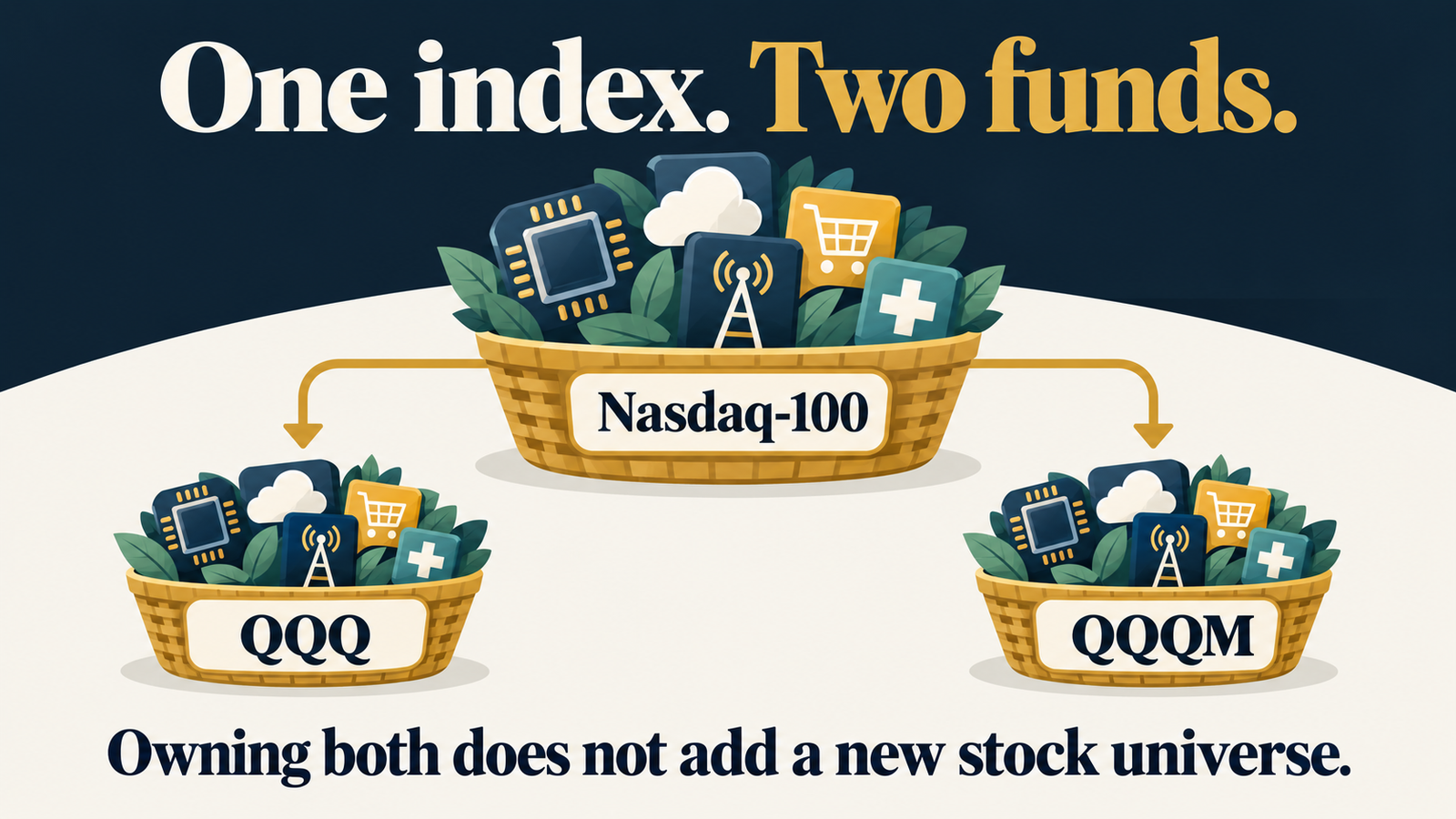
QQQ and QQQM both seek exposure to the Nasdaq-100. Their common benchmark is the reason the expense comparison is meaningful. You are not exchanging a broad global portfolio for a different asset class; you are comparing two ways to access a substantially shared stock universe.
The Nasdaq-100 contains large non-financial companies listed on Nasdaq, subject to its methodology. It is different from the Nasdaq Composite and from a total U.S. market benchmark. Its holdings and weights can create concentrations that should be reviewed in the context of your other investments.
A lower expense ratio does not make an unwanted allocation suitable. If your actual concern is too much exposure to a handful of large businesses, changing between these vehicles may leave the central issue in place. Calculate the resulting portfolio allocation before describing the switch as diversification.
Separate two decisions in your notes: whether the benchmark fits the portfolio, and which fund implementation suits the intended holding and trading pattern. Doing that keeps the three-basis-point difference from becoming a substitute for the larger investment decision.
Translate the fee difference into dollars
Three basis points equals 0.0003 as a decimal multiplier. Multiply the constant position value by that figure to estimate a year’s expense difference. A $10,000 position produces approximately $3; $50,000 produces $15; $100,000 produces $30.
| Position | QQQ at 0.18% | QQQM at 0.15% | Difference |
|---|---|---|---|
| $10,000 | $18 | $15 | $3 |
| $50,000 | $90 | $75 | $15 |
| $100,000 | $180 | $150 | $30 |
An expense ratio relates operating expenses to fund assets. The illustration is not a promise of an exact annual debit from your brokerage cash. Expenses are reflected in fund assets and results, and the dollars vary as the position value and holding period change.
Older articles may use a 0.20% QQQ fee. Invesco’s current explanation describes the reduction to 0.18% alongside its move to an open-ended structure. Using 0.20% would overstate the current fee gap and make the apparent recovery period shorter than the present inputs justify.
Published fund returns generally already reflect operating expenses. If you compare those returns, do not subtract the expense ratios again. For this guide’s fee-only worksheet, we instead isolate the operating-cost difference without pretending that it guarantees an equal realized-performance advantage.
Define the switching cost before calculating recovery

List the costs attached to the proposed sale and purchase. Include commissions on both legs, an estimate of execution friction and any relevant currency or account charges. Record where each estimate came from and whether the broker has already included it in another number.
A bid-ask spread needs careful interpretation. If you estimate transaction cost relative to a midpoint, selling at the bid and buying at the ask each involve a half-spread in a simplified symmetric quote. Adding the full spread for each leg as well can double count friction. Actual execution can differ from either assumption.
For an invented $50,000 transition, suppose commissions total $10, sale-side estimated friction is $12 and purchase-side friction is $8. The assumed direct cost is $30. At $15 of annual fee savings, simple recovery takes two years if asset value and fees remain constant.
Timing risk is not captured by that estimate. If the sale and purchase occur at different times, market movement can alter the result. A limit order controls an acceptable price but may not fill. The calculator does not assume that a broker can complete the exchange instantly at identical underlying values.
Use a plausible range when the quote or execution cost is uncertain. Testing $20, $40 and $80 is more informative than entering one precise-looking estimate unsupported by a quote. The purpose is to see which assumptions could change the decision.
Three original cases show the scale of the decision
First consider an invented $100,000 position with $30 of assumed total direct transition costs. Annual fee savings are $30 under current ratio inputs. The simple recovery period is one year. Over a five-year constant-value horizon, accumulated gross fee savings are $150 and the modeled amount after the transition cost is $120.
Next consider a $10,000 position with the same $30 transition cost. Annual fee savings are $3, so simple recovery takes ten years. Over five years the worksheet shows $15 of gross savings and a negative $15 amount after the cost. The same fee percentages produce a different practical result because the fixed cost consumes more of the smaller position.
Finally consider a $50,000 position and $45 of direct costs. The simple recovery period is three years. If an additional $300 of tax cash outflow is included as a sensitivity assumption, total modeled outflow becomes $345 and the recovery period becomes twenty-three years.
The third case is deliberately limited. It does not say that a $300 tax payment is the full economic cost of a taxable sale. Tax timing, adjusted cost basis, future sales and account rules can change that analysis. It shows why an unexamined tax consequence can dwarf a small annual fee difference.
Each case uses constant value, unchanged fees and no compounding. The model is a transparent first screen. A result that looks attractive under that screen still deserves an implementation review, while an unattractive result can identify the assumption worth investigating next.
Keep tax timing separate from the fee-only model
A sale can have account- and jurisdiction-specific consequences. The worksheet needs your relevant cost records and current rules; the fund ticker alone cannot tell you the tax result. A retirement account, a taxable account and an account held in another country can require different analysis.
Do not mechanically multiply an unrealized gain by a guessed tax rate and call the result the permanent cost of switching. The sale may accelerate a payment that otherwise would occur later, change the remaining tax basis or interact with other gains, losses and deductions. Timing has value and should be evaluated explicitly.
For an initial sensitivity test, the calculator lets you include an assumed immediate tax cash outflow. Label it as such. Its effect on the recovery period shows whether tax questions are material enough to justify a fuller account-specific comparison before placing orders.
If the sale realizes a loss, replacement-security and loss-recognition rules can also matter. This guide does not determine whether a particular replacement qualifies under any country’s rules. Check the applicable treatment rather than inferring it from shared index exposure.
Where tax uncertainty dominates the arithmetic, resolve that uncertainty first. Three basis points of annual cost difference is a modest benefit; a larger unverified assumption should not be hidden inside the spreadsheet simply because the expense ratios are easy to find.
Stress-test the holding horizon and position value
The planned holding period should reflect your actual strategy. A five-year horizon written to justify the trade has little value if you usually replace the position every few months. Use several horizons to see whether the apparent benefit depends on unusually long uninterrupted ownership.
The constant-value assumption is another important limit. If the position falls from $50,000 to $30,000 and remains there, a three-basis-point gap represents $9 annually, rather than $15. With a $45 starting cost, recovery under that revised constant-value scenario is five years.
If the position instead grows to a constant $80,000, the gap represents $24 annually and the same cost recovers in approximately 1.88 years. Neither scenario predicts the market. They demonstrate why a starting-value estimate is a scale check rather than a guarantee.
Fee schedules can change too. Equal future expense ratios would eliminate the modeled recurring advantage. A lower replacement ratio is therefore an assumption to revisit, not a permanent contractual spread promised to the investor.
Compare a full switch with future purchases

Buying QQQM with future contributions does not require selling the existing QQQ position. That can avoid a sale-related cost on the old holding while allowing new money to use the preferred vehicle. It still creates two positions with substantially shared exposure, which should be combined in portfolio reviews.
For a household unable to add contributions, available cash and distributions may be the only source for incremental purchases. Whole-share restrictions can delay purchases or leave residual cash. A lower price per unit can affect implementation without establishing that the underlying stocks are cheaper.
Investors who use options, frequent trades or large orders need to review those requirements separately. Existing contracts and the exact securities needed to support them can constrain a transition. The operating-expense calculation does not price closing a derivative position or rebuilding a trading arrangement.
Use current quotes, order sizes and broker charges for an actual proposal. Record the intended sale and purchase, the estimated combined friction and what happens if one leg fills and the other does not. A workable operational plan is part of assessing the benefit.
Common questions about switching from QQQ to QQQM
Does the lower fee guarantee better realized returns?
No. A fee difference is one component of implementation. Tracking, cash balances, execution and market movement can affect realized results. The calculator isolates one cost relationship rather than forecasting performance.
What if switching has no cost?
With a positive annual expense difference and zero assumed outflow, the simple model shows immediate cost recovery. Still review the exposure and implementation assumptions; a zero commission alone does not establish zero total cost.
What if the replacement expense ratio is equal or higher?
There is no positive recurring fee saving under those inputs. The tool displays no fee-based recovery period rather than dividing by zero or presenting a negative recovery time as a benefit.
Can I keep QQQ and use QQQM for new money?
That is a separate implementation option if the account permits it. Include both positions when reviewing concentration and maintenance, and do not count them as independent stock universes.
Switching from QQQ to QQQM: cost-recovery calculator
Compare the cost with your holding horizon
Under the selected assumptions, modeled savings exceed the one-time outflow over five years.
Annual savings = position × (current ratio − replacement ratio) ÷ 100. Simple recovery = one-time outflow ÷ positive annual savings. Horizon result = annual savings × years − outflow. Assumes constant position value and fees; no compounding, contributions, market movement or tracking differences. Tax input is an optional cash-flow sensitivity, not tax advice or a full economic comparison. All amounts use the same currency.
Continue Learning in the Invest & Compound Academy
Put this cost-recovery decision in context with our related ETF research guides.
References & Official Data Sources
Expense ratios and shared benchmark descriptions were reviewed October 5, 2026 using Invesco materials. Quotes, tax amounts, costs and scenarios in this guide are hypothetical. For a broader introduction, see QQQ versus QQQM and our ETF research guide.
- Invesco: QQQ’s current structure and 0.18% expense ratio
- Invesco: QQQM objective and 0.15% expense ratio
- Invesco: QQQM fact sheet