How Long Do Bear Markets Last? Historical Evidence and Recovery Times
Understand what historical averages measure, why recovery can take longer than the decline, and how withdrawals change the capital available for a rebound.
How long do bear markets last? When stock markets enter bear-market territory, investors want to know how much further prices could fall and how long the downturn could continue. The first question concerns the potential severity of the decline. The second concerns something equally important: the amount of time an investor may need to remain financially and psychologically prepared for unfavorable market conditions. Bear markets are conventionally defined as declines of at least 20% from a previous market high. However, that definition reveals almost nothing about their eventual duration.
Some bear markets develop in a matter of weeks. Others continue for more than a year. The time required for a market to regain its previous high can extend considerably beyond the period of falling prices. Historical research provides useful perspective, but it also reveals significant differences between market downturns. According to Hartford Funds, using research from Ned Davis Research with a table covering 1929 through 2024, the average S&P 500 bear-market episode lasted approximately 289 calendar days, equivalent to about 9.6 months, from peak to trough.
That same dataset reports an average price decline of approximately 35%. These findings offer a historical reference, not a forecast. The next bear market could be considerably shorter or longer than the average. Its severity may differ substantially from previous downturns, and its recovery may be influenced by economic forces not present in earlier periods. More importantly, the 289-day average refers to the decline phase under a particular market-cycle methodology. It does not mean investors typically regain their original portfolio values within 289 days. Recovery is a separate process.
A market can fall 30% over several months and require years to regain its previous peak. Another market may lose a similar amount within weeks and rebound much more quickly. For investors building wealth over decades, understanding this distinction is essential. It influences asset allocation, retirement planning, liquidity reserves, investment expectations, and the financial capacity to remain invested during prolonged uncertainty. This guide examines historical bear-market durations, major U.S. downturns, the mathematics of investment recovery, and the forces that influence how long market weakness can continue.
It also explains why bear markets cannot be accurately timed using simple historical averages—and how investors can use the available evidence to build more resilient financial strategies.
What Is a Bear Market?
A bear market occurs when the value of a market index or financial asset declines at least 20% from a relevant previous peak. For broad U.S. equities, the S&P 500 is frequently used as the benchmark for identifying bear-market episodes. Suppose the index reaches 6,000 points. A subsequent decline to 4,800 represents a 20% loss. The calculation is:
Using the example:
The conventional bear-market threshold has been reached. However, this threshold describes the size of the decline rather than its cause or duration. A bear market can develop during an economic recession, but a recession is not required. A decline may result from changing interest-rate expectations, collapsing valuations, deteriorating corporate earnings, financial-system stress, or an unexpected global event. The distinction matters because different catalysts can produce very different recovery patterns. A temporary disruption to business activity may resolve more quickly than a prolonged banking crisis or a major adjustment following years of speculative overvaluation.
Why the Definition Requires Consistent Measurement
Financial researchers do not always classify bear markets using identical methods. Some measure declines using daily closing prices. Others incorporate intraday values. Some treat a substantial rebound of 20% from a trough as the beginning of a new bull market. Others organize historical data into broader peak-to-trough and peak-to-recovery cycles. These choices affect the number of bear markets counted and the calculated average duration. For example, a prolonged decline involving several large rebounds might be classified as one extended bear market in one dataset and multiple bear-market legs in another. Neither approach is automatically invalid.
The important requirement is to understand what each statistic actually measures.
For causes and mechanics, see our bear-market guide. Our market correction vs bear market comparison explains the classification boundary; this article concentrates on historical duration and recovery.
What Is the Average Length of a Bear Market?
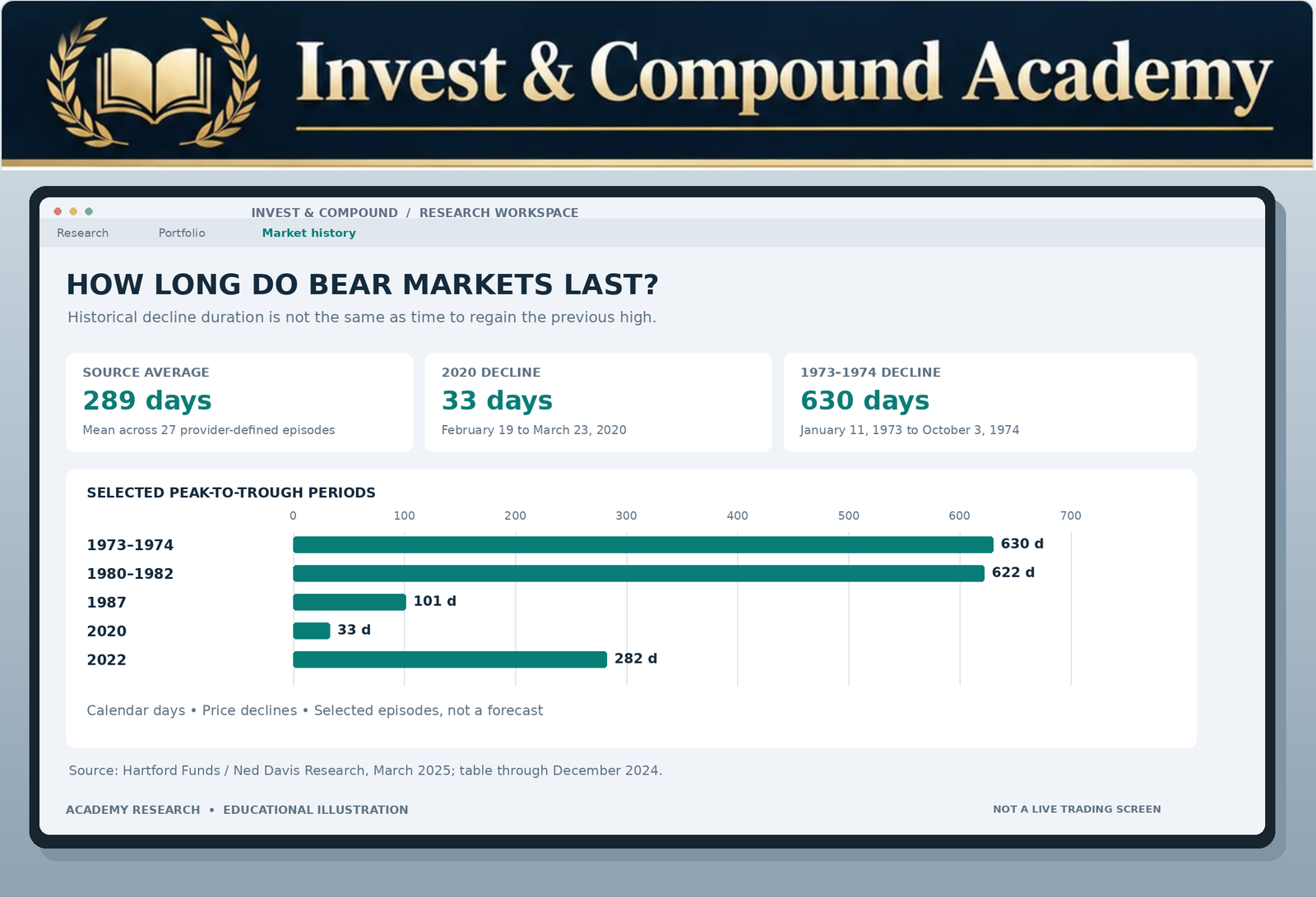
Hartford Funds’ published historical analysis reports that S&P 500 bear markets averaged approximately 289 calendar days from peak to trough in its table covering 1929–2024. The corresponding average price decline was approximately 35.24%. The dataset identifies 27 bear-market episodes. These figures are based on research from Ned Davis Research, with the underlying statistics updated in March 2025. The average duration is therefore approximately nine and a half months. However, investors should not interpret this as a countdown. A bear market reaching its seventh month is not automatically approaching its end.
Nor does a market recovering after only six weeks violate any statistical rule. An average summarizes historical observations. It does not impose a schedule on future financial markets.
Average Duration Versus Median Duration
The arithmetic average is calculated by adding the durations of all observations and dividing by the number of observations. The median identifies the middle observation after durations are arranged from shortest to longest. The distinction matters because unusually prolonged downturns can pull the average higher. Consider seven hypothetical bear markets lasting: 35, 90, 130, 210, 280, 400, and 900 days. The average duration is approximately 292 days. The median is only 210 days. The unusually long 900-day episode significantly influences the mean. Historical investment data frequently contain extreme observations.
This makes averages useful for broad comparisons but insufficient for estimating the likely duration of a specific future event.
Why Historical Data Cannot Predict the Next Bear Market
Financial markets are not governed by a fixed cycle that causes a bear market to end after a predetermined number of days. Each downturn develops under a particular combination of economic conditions, market valuations, policy decisions, corporate earnings, and investor positioning. These conditions change over time. The banking system today operates under different regulations and institutional arrangements from those present in the 1930s. The role of exchange-traded funds, algorithmic trading, derivatives, global capital flows, and monetary policy has also evolved.
Historical observations remain valuable, but their statistical distribution should not be treated as an exact description of future probabilities.
Source: Hartford Funds / Ned Davis Research, table through December 2024 and source dated March 2025. The last qualifying bear episode in that table is 2022. The published 9.6-month equivalent uses an approximate month length.
The Difference Between Bear-Market Duration and Recovery Time
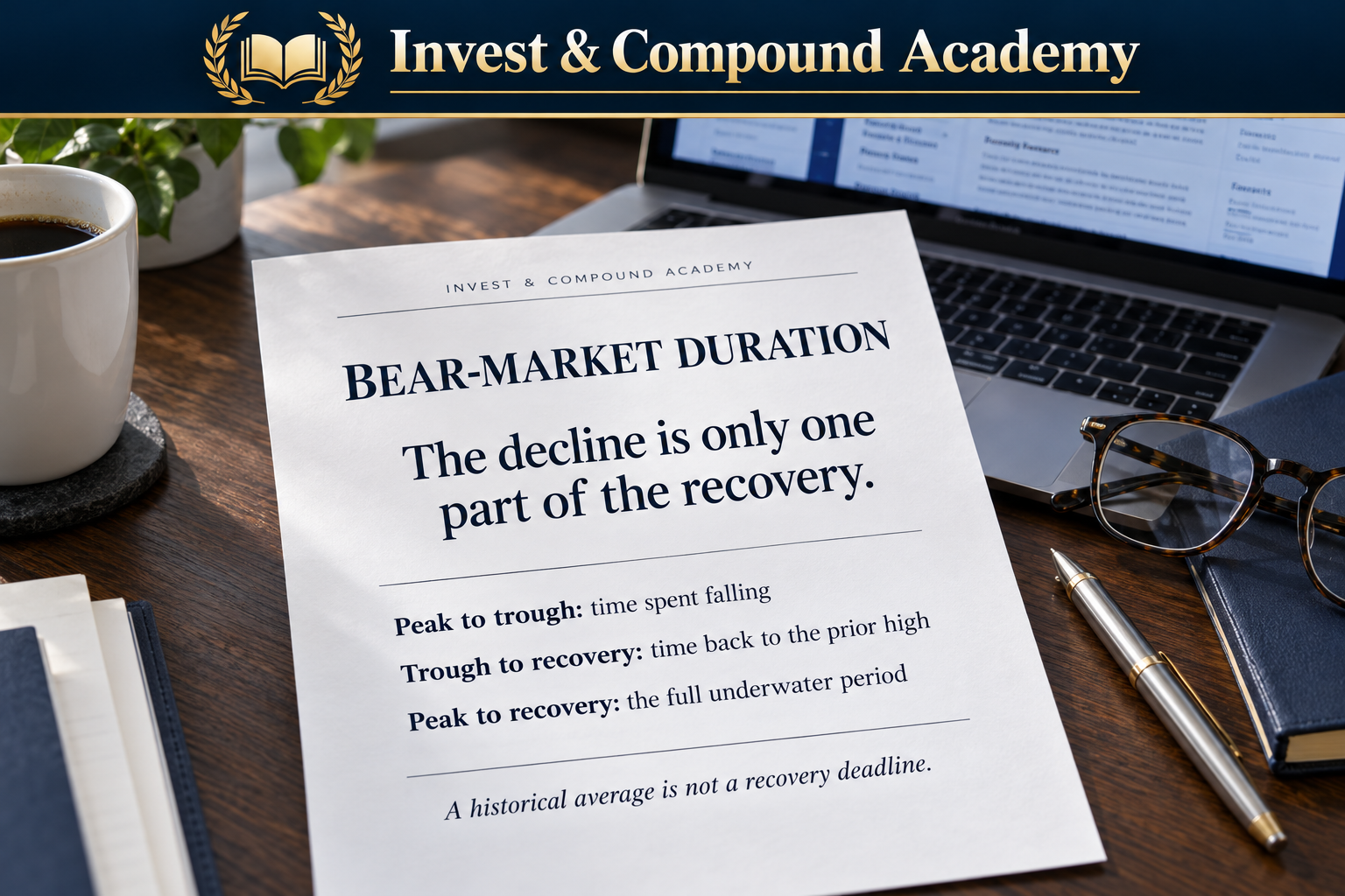
One of the most common mistakes in discussions of bear-market history is treating the duration of the decline as equivalent to the time required for investors to recover. They are different measurements.
Peak-to-Trough Duration
Peak-to-trough duration measures the time between the previous market high and the subsequent lowest value. This is the period during which the maximum drawdown develops. For example, suppose an index reaches 5,000 in January and declines to 3,500 by October. The market has fallen 30%. The decline phase lasted approximately nine months. This is the type of measurement reflected in the Hartford Funds 289-day historical average.
Trough-to-Recovery Duration
Trough-to-recovery duration measures how long the market takes to regain the previous high after reaching its lowest point. Continuing the example, suppose the index reaches 3,500 in October but does not return to 5,000 until the following December. The recovery phase lasted approximately fourteen additional months. Although selling pressure reached its maximum effect during the first nine months, investors had to wait much longer for the index to regain the original peak.
Peak-to-Recovery Duration
Peak-to-recovery duration combines the decline and rebound periods. In the example, the complete underwater period lasted approximately twenty-three months. This can be particularly relevant for investors who held the index through the entire episode. The original peak represents the value their portfolio had achieved before the downturn. However, an individual’s actual recovery date may differ because of contributions, withdrawals, dividends, fees, taxes, and investment selection.
Comparing the Measurements
| Measurement | Begins | Ends | What it tells investors |
|---|---|---|---|
| Peak-to-trough | Previous high | Lowest subsequent level | How long prices declined |
| Trough-to-recovery | Market low | Previous high regained | How long the rebound took |
| Peak-to-recovery | Previous high | Previous high regained | Total time below the previous peak |
The same market episode can therefore produce several legitimate duration statistics. Whenever a research report describes a bear market lasting a particular number of months, the first question should be: Which of these periods is being measured?
For smaller downturns, compare how long market corrections last. Our market-correction pillar covers their broader mechanics.
Historical Bear Markets in the S&P 500
U.S. equity-market history provides a wide range of bear-market experiences. Some declines were relatively brief but extremely severe. Others developed gradually over hundreds of days. Hartford Funds’ historical table, based on Ned Davis Research, provides a consistent illustration of this variation. The following entries are selected from that source’s bear-market classification.
Selected Historical Bear-Market Episodes
| Episode | Peak-to-trough dates | Price decline | Duration |
|---|---|---|---|
| 1968–1970 | Nov. 29, 1968–May 26, 1970 | −36.06% | 543 days |
| 1973–1974 | Jan. 11, 1973–Oct. 3, 1974 | −48.20% | 630 days |
| 1980–1982 | Nov. 28, 1980–Aug. 12, 1982 | −27.11% | 622 days |
| 1987 | Aug. 25–Dec. 4, 1987 | −33.51% | 101 days |
| 2000–2001 segment | Mar. 24, 2000–Sept. 21, 2001 | −36.77% | 546 days |
| 2002 segment | Jan. 4–Oct. 9, 2002 | −33.75% | 278 days |
| 2007–2008 segment | Oct. 9, 2007–Nov. 20, 2008 | −51.93% | 408 days |
| Early 2009 segment | Jan. 6–Mar. 9, 2009 | −27.62% | 62 days |
| 2020 | Feb. 19–Mar. 23, 2020 | −33.92% | 33 days |
| 2022 | Jan. 3–Oct. 12, 2022 | −25.43% | 282 days |
Source: Hartford Funds, based on Ned Davis Research data updated March 2025. Durations are calendar days. These represent the provider’s classification of separate bear-market legs; some entries do not represent the full uninterrupted drawdown from an earlier all-time high.
The table illustrates enormous variation in duration. The 2020 episode lasted just 33 days from peak to trough. The 1973–1974 bear market lasted approximately 630 days under the same published classification. The difference reflects distinct economic circumstances and market dynamics. It does not establish that faster declines necessarily recover faster.
For benchmark construction, read how the S&P 500 works. Historical series before the index’s 1957 launch use predecessor or reconstructed history; they are not observations of a live 500-stock index at that time.
Why Some Historical Sources Report Different Bear-Market Durations
Market-history statistics can appear contradictory when researchers use different cycle definitions. The 2000–2002 technology collapse provides a useful illustration. Under a broad peak-to-trough perspective, investors often describe the downturn as extending from the market’s 2000 high through the 2002 low. However, the Hartford Funds table separates the broader period into a 2000–2001 bear-market segment and another segment during 2002. Similarly, the 2007–2009 financial crisis appears as separate 2007–2008 and early-2009 declines in that dataset.
Splitting one prolonged historical downturn into shorter episodes changes the number of observations and therefore affects average duration. A researcher using a different convention may combine those movements into a longer drawdown. That study would produce different statistics even when examining closely related market data.
A Hypothetical Illustration
Imagine a market peaks at 100 and declines to 75 over six months. It then rallies to 92 before falling to 60 over another five months. One methodology may treat the complete move from 100 to 60 as a single broader 40% drawdown. Another approach using specific rules for identifying new bull and bear phases may divide the history differently if its rebound conditions are satisfied. The resulting duration statistics would not necessarily match.
For educational research, the appropriate response is to disclose the methodology. Historical market data require interpretation; they are not universally interchangeable numbers.
The 1929–1932 Great Depression Market Collapse
The Great Depression provides one of the most severe examples of prolonged financial-market distress. The U.S. equity market experienced extraordinary losses following the 1929 peak. The Dow Jones Industrial Average fell approximately 89% from its September 1929 peak to its July 1932 low. The decline was accompanied by severe banking instability, falling output, widespread unemployment, and a collapse in business confidence. It is important to distinguish the overall economic and market collapse from the separate bear-market legs reported in certain historical datasets. Hartford Funds’ methodology identifies multiple substantial declines during the broader 1929–1932 period.
This reflects the occurrence of significant rebounds within a longer crisis.
Why the Collapse Lasted So Long
The economic environment involved persistent financial-system problems rather than a brief disappointment in corporate earnings. Bank failures reduced confidence and impaired credit intermediation. Falling asset prices weakened collateral values. Businesses faced deteriorating demand. Household finances came under enormous pressure. Deflation increased the real burden of many outstanding debts. These interacting forces reinforced the downturn.
What Investors Can Learn
The Great Depression demonstrates why bear markets cannot be evaluated solely through changes in stock prices. Financial institutions, credit availability, economic production, and household income can all influence the market’s capacity to recover. However, comparisons with the 1930s must recognize major institutional differences. Modern deposit insurance arrangements, central-bank practices, financial regulation, and government policy frameworks differ substantially from those of the Great Depression era.
Severe economic imbalances can prolong financial-market weakness beyond what investors initially expect. The experience does not imply that every bear market will resemble the 1930s.
The 1973–1974 Bear Market
The 1973–1974 market decline occurred during an environment characterized by inflation, economic uncertainty, and major energy-price disruptions. The S&P 500 experienced a substantial decline. Hartford Funds’ historical dataset identifies a peak-to-trough period of 630 calendar days and a price loss of approximately 48.2%. This makes the episode a useful example of a prolonged bear market involving multiple economic pressures.
Inflation and Valuation Pressure
High inflation affects the economy through several channels. Businesses may face rising labor, transportation, and input costs. Consumers can experience reduced purchasing power. Central banks may maintain restrictive monetary conditions. Higher required returns can place downward pressure on equity valuation multiples. The combination of weaker expected earnings and lower valuation multiples can generate substantial stock-market losses.
The Importance of Real Returns
During inflationary periods, investors must distinguish between nominal and inflation-adjusted investment results. Suppose a portfolio falls from $100,000 to $70,000 and subsequently recovers to $100,000. In nominal terms, the investor has regained the original amount. However, if the general price level has increased by 20% over the complete period, the recovered $100,000 does not purchase the same quantity of goods and services. Its purchasing power relative to the initial period is approximately $83,333. This demonstrates why nominal recovery does not necessarily mean complete economic recovery.
Investors evaluating historical market outcomes should consider inflation alongside market prices.
The 1980–1982 Bear Market
The early 1980s illustrate another difficult environment for financial markets. The United States experienced severe inflationary pressures and restrictive monetary policy. Interest rates reached unusually high levels as policymakers attempted to restore price stability. The period also included economic recessions. Hartford Funds’ bear-market table records a decline of approximately 27.1% over 622 calendar days beginning in November 1980. The duration demonstrates that a bear market does not need to produce an exceptionally large percentage loss to continue for a prolonged period.
Why Monetary Policy Matters
Interest rates influence the cost of borrowing and the valuation of future cash flows. When rates rise, companies may face higher financing costs. Consumers may reduce interest-sensitive spending. Investors may demand higher returns for holding risky assets. These developments can place pressure on equity prices. However, changes in monetary policy do not have an immediate or uniform effect on every company. Businesses differ in their sensitivity to credit costs, consumer demand, and the economic cycle.
The Lesson for Investors
Prolonged financial-market weakness can occur while policymakers are addressing deeper economic imbalances. An investor relying on the assumption that lower stock prices will produce a rapid recovery may underestimate the time needed for those imbalances to improve.
The 1987 Stock Market Crash
The 1987 crash illustrates the opposite extreme: a severe market decline developing over a relatively short period. Hartford Funds’ dataset records a bear-market episode lasting 101 calendar days, with a decline of approximately 33.5%. On October 19, 1987, the Dow Jones Industrial Average fell approximately 22.6% in a single trading session. The event involved changes in market expectations, trading mechanisms, portfolio insurance strategies, and liquidity pressures.
Why the Speed Was Extraordinary
Financial markets can respond rapidly when many participants attempt to reduce risk simultaneously. Selling pressure may become self-reinforcing. Price declines can trigger additional transactions, increasing volatility. The speed of a downturn can therefore reflect trading structure and liquidity conditions, not only changes in expected corporate earnings.
Why 1987 Matters for Duration Analysis
The 1987 experience demonstrates that severe losses are not necessarily associated with prolonged peak-to-trough periods. A market can enter bear-market territory very rapidly. However, a short decline phase does not automatically guarantee an immediate return to the previous peak. Investors must examine both the fall and the subsequent recovery. The event also illustrates why maintaining adequate liquidity and avoiding unsuitable leverage can matter even when financial markets appear relatively stable.
The 2000–2002 Technology Bear Market
The collapse following the late-1990s technology boom provides a particularly important lesson about valuations and prolonged recovery. During the expansion, investors became highly optimistic about internet businesses, telecommunications infrastructure, and the commercial potential of emerging technologies. Some companies generated strong operating growth. Others traded at extraordinary valuations despite limited profits or uncertain business models. When expectations changed, share prices declined substantially. The broader S&P 500 entered a prolonged bear market, while the Nasdaq Composite experienced even deeper losses.
Why the Decline Continued
The downturn involved more than a temporary change in investor sentiment. Corporate profit expectations deteriorated. Business investment weakened in several technology-related industries. Companies that had depended on continued capital-market access faced increasing financial pressure. The market also needed to reassess valuations that had reflected exceptionally optimistic forecasts.
Recovery Was Uneven
A broad market index and an individual technology company can experience very different recovery patterns. Some companies eventually became highly profitable. Others disappeared, were acquired at depressed valuations, or failed to regain previous market prices. Consequently, a broad index’s historical recovery does not imply that every security held during the downturn recovered.
What the Episode Demonstrates
Valuation risk can persist for years. A company may participate in a promising industry and still prove to be an unattractive investment when purchased at an excessive price. Investors should distinguish technological progress, business growth, profitability, and shareholder returns. These concepts are related but not interchangeable.
The 2007–2009 Global Financial Crisis
The global financial crisis provides a major example of financial-system stress producing a severe and prolonged market downturn. The S&P 500 reached a market high in October 2007. The subsequent decline developed alongside problems in housing-related credit, financial institutions, and the broader economy. The market eventually reached its major low in March 2009. The closing-price decline from the earlier peak was approximately 57%.
Why the Crisis Was Different
The downturn involved substantial deterioration in financial intermediation. Bank balance sheets faced pressure. Investors became increasingly concerned about the value of complex credit instruments. Access to financing deteriorated. Corporate and household confidence weakened. These developments created feedback effects between financial markets and economic activity.
A Bear Market With Multiple Legs
Hartford Funds’ Ned Davis Research dataset identifies two separate bear-market legs within the broader financial-crisis period. The first extends from October 2007 to November 2008. The second covers early January through March 2009. By contrast, a full peak-to-trough analysis of the 2007–2009 crisis generally treats the market’s decline from the October 2007 high to the March 2009 low as a broader drawdown. The distinction is important when comparing reported durations.
An investor who held an S&P 500 index investment throughout the broader collapse experienced the cumulative effect of the entire peak-to-trough decline, regardless of how a particular research methodology divided the period.
The Recovery Challenge
Following the March 2009 trough, equities began a sustained recovery. However, regaining the previous 2007 price-index high took several years. The distinction between reaching a market low and returning to the previous peak was substantial. For investors who needed to withdraw capital during the intervening period, the consequences could be especially serious. The crisis demonstrates why recovery duration should be considered alongside drawdown severity, liquidity, and financial obligations.
The 2020 Pandemic Bear Market
The pandemic bear market stands out for its extraordinary speed. The S&P 500 reached a peak on February 19, 2020. It fell sharply as investors assessed the economic consequences of COVID-19. The index reached its trough on March 23, 2020. Hartford Funds’ dataset records a peak-to-trough decline of approximately 33.9% over just 33 calendar days.
Why the Decline Happened So Quickly
The pandemic created immediate uncertainty about economic activity. Travel restrictions, temporary business closures, disrupted supply chains, and changes in consumer behavior affected many industries. Investors rapidly reduced expectations for near-term corporate earnings. Financial markets also experienced significant liquidity pressure.
Why the Recovery Was Relatively Rapid
The subsequent market recovery was influenced by extraordinary fiscal and monetary measures, changes in investor expectations, and adaptation across parts of the economy. The S&P 500 regained its previous price-index high later in 2020. The full recovery occurred far more quickly than many investors initially expected. However, the recovery was not equally distributed across companies and industries. Some businesses benefited from changes in consumer behavior and digital adoption. Others faced prolonged operational disruption.
Why 2020 Should Not Be Treated as a Universal Model
The speed of the 2020 recovery reflected a particular set of circumstances. It does not establish that future bear markets must recover within months. A downturn involving prolonged inflation, impaired credit markets, or deep structural problems could follow a very different path. Investors who assume every bear market will resemble 2020 risk underestimating the possibility of extended weakness.
The 2022 Bear Market
The 2022 bear market was driven substantially by inflation, higher interest rates, tighter monetary policy, and changing valuations. The Federal Reserve raised interest rates aggressively as it responded to persistent inflationary pressures. Higher discount rates affected the valuation of future corporate cash flows. Growth-oriented companies were particularly sensitive in many parts of the market. The S&P 500 entered bear-market territory. Hartford Funds’ historical table identifies the January 3–October 12, 2022, episode as lasting 282 calendar days, with a price decline of approximately 25.4%.
Why Stocks and Bonds Both Faced Pressure
Diversified investors sometimes expect bonds to offset equity-market losses. However, bonds and stocks can decline together when interest rates rise sharply. Bond prices generally move inversely to yields, all else being equal. Higher required returns can also put pressure on equity valuation multiples. As a result, investors holding traditional stock-and-bond portfolios experienced a challenging environment.
Why the 2022 Episode Matters
The episode demonstrates that bear markets do not require a banking crisis or pandemic. A significant shift in the interest-rate environment can produce substantial losses. It also illustrates why portfolio diversification should be based on the actual economic risks represented by different assets rather than assuming historical correlations will remain constant.
How Long Does It Take to Recover From a Bear Market?
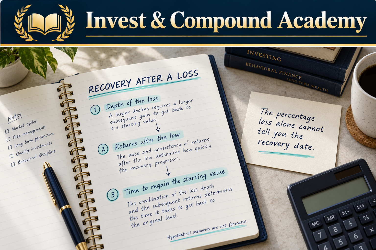
The period required to regain a previous market high varies considerably. It depends on the depth of the decline, subsequent returns, economic conditions, valuations, and the index being measured. A market falling 20% needs to gain 25% to recover. A market falling 40% needs to gain approximately 66.67%. A market falling 50% needs to double. The recovery becomes mathematically more demanding as the drawdown deepens.
Recovery Formula
Required Returns After Different Bear-Market Losses
| Drawdown | Remaining value of $100,000 | Required recovery gain |
|---|---|---|
| 20% | $80,000 | 25.00% |
| 25% | $75,000 | 33.33% |
| 30% | $70,000 | 42.86% |
| 35% | $65,000 | 53.85% |
| 40% | $60,000 | 66.67% |
| 45% | $55,000 | 81.82% |
| 50% | $50,000 | 100.00% |
| 60% | $40,000 | 150.00% |
The figures assume no contributions, withdrawals, fees, distributions, or taxes.
Why a Larger Required Gain Does Not Establish Recovery Time
Consider two hypothetical markets. Market A falls 40% and subsequently generates strong gains over several years. Market B falls only 22% but experiences a prolonged period of weak positive and negative returns. Market A may recover faster despite its deeper initial decline. The amount of the required gain affects the challenge, but the pace of future returns determines the actual recovery period.
How Annual Returns Affect Recovery Time
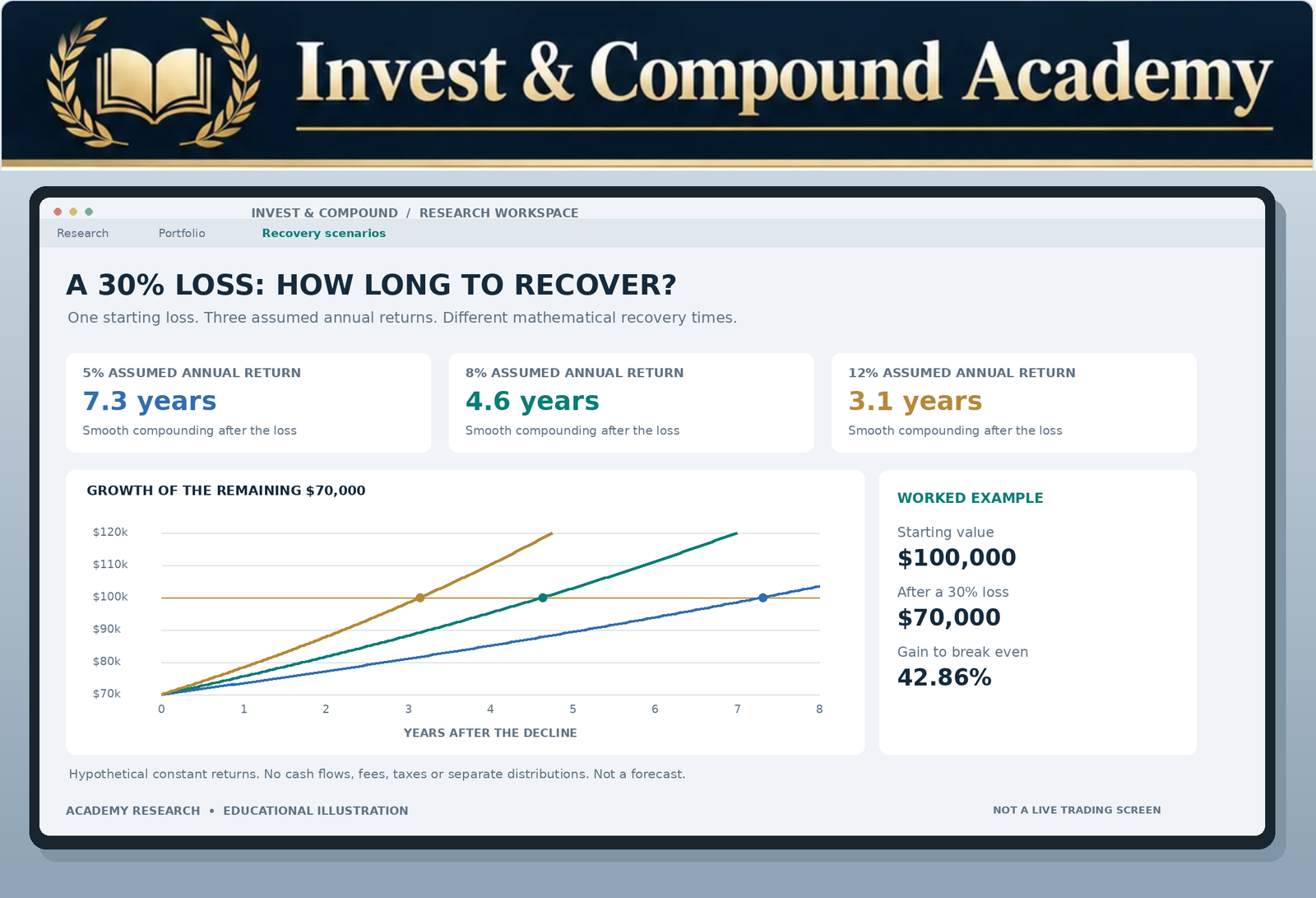
An illustrative calculation can help demonstrate the relationship between drawdown severity and subsequent growth. Suppose a portfolio begins at $100,000 and falls 30%. Its value becomes $70,000. The investor needs a total return of approximately 42.86% to recover. If the portfolio subsequently earns a constant annual compounded return of 5%, recovery would take approximately 7.3 years. At 8% annually, recovery would take approximately 4.6 years. At 12% annually, recovery would take approximately 3.1 years. These calculations use a mathematical model assuming constant positive annual returns after the decline.
Real market performance does not follow a smooth schedule. Returns fluctuate, and negative years may occur during recovery. The purpose of the example is to illustrate sensitivity to the growth rate, not to forecast how quickly stocks will rebound.
Recovery Time Formula
For a constant positive compound growth rate:
Where ln represents the natural logarithm. This formula can be used in a recovery-time calculator. However, it is important to disclose that the result assumes a fixed annual growth rate. It does not incorporate market volatility, changing contributions, distributions, taxes, or fees.
Why Bear Markets Sometimes Recover Before Recessions End
Financial markets are forward-looking. Investors value assets based on expectations about future earnings, cash flows, and required returns. Economic statistics often describe activity that has already occurred. As a result, the stock market can begin recovering while the economy remains weak. Suppose investors initially expect corporate earnings to decline 30%. Stock prices fall as those expectations are incorporated into valuations. Later, new information suggests that earnings may decline only 15%. Even though the outlook remains unfavorable in absolute terms, it is better than the market previously anticipated. Equity prices may rise.
This explains why investors who wait for uniformly positive economic headlines may miss part of a recovery.
Recessions and Bear Markets Are Different Measures
A recession describes a contraction in economic activity. In the United States, the National Bureau of Economic Research identifies business-cycle peaks and troughs using several economy-wide indicators. A bear market describes a decline in financial asset prices. These events may overlap, but their dates are not necessarily identical. The NBER identifies the 2007–2009 recession as lasting from December 2007 through June 2009. The broad S&P 500 market decline reached its low in March 2009, before the officially dated recession trough. This illustrates how market prices can begin recovering ahead of an economic turning point.
It also highlights why recession-duration statistics should not be substituted for bear-market duration statistics.
How Interest Rates Influence Bear-Market Duration
Monetary policy can influence financial markets through several channels. Higher interest rates generally increase borrowing costs and the discount rates applied to future cash flows. This can affect both economic activity and asset valuations. When monetary conditions tighten, companies may face higher financing expenses. Consumers may reduce spending on credit-sensitive purchases. Investors may demand higher expected returns from risky assets. These forces can contribute to prolonged market weakness. However, lower interest rates do not automatically bring a bear market to an end.
Why Rate Cuts Can Coincide With Falling Stocks
Central banks sometimes lower rates because economic conditions are deteriorating. If earnings expectations are falling rapidly or financial stress is increasing, equities may continue declining despite lower policy rates. Investors should therefore distinguish between the direction of interest rates and the reasons monetary policy is changing.
The Role of Financial Conditions
Credit spreads, lending standards, liquidity, and refinancing conditions also influence market outcomes. Improvement in these areas can support a recovery. Deterioration can extend market weakness even when some headline indicators appear more favorable. Bear-market analysis should therefore examine the broader financing environment rather than interest rates alone.
Do Bear Markets Last Longer When Valuations Are High?
High starting valuations can increase vulnerability to disappointing future performance. When investors pay unusually high prices for expected earnings, the market may have less tolerance for weaker growth or higher interest rates. A company initially valued at 40 times earnings may experience substantial losses if investors eventually value it at 25 times earnings. However, valuation alone does not establish the timing or duration of a bear market. Expensive markets can continue rising. Cheap markets can remain depressed.
A Numerical Example
Suppose a company earns $5 per share and trades at 40 times earnings. Its share price is $200. Investors subsequently reduce the valuation multiple to 25. With earnings unchanged, the implied price becomes $125. The decline is 37.5%. If future earnings forecasts also weaken, the loss could become larger. This illustrates how valuation compression can contribute to a bear market even without a proportional decline in corporate profitability.
Why Valuation Is More Useful for Long-Term Analysis
Valuation measures can help investors evaluate prospective returns and risk. They are generally less reliable as short-term timing signals. The market can remain above or below estimated fair value for extended periods. Investors should therefore be cautious about using one valuation ratio to predict the date of the next market bottom.
The P/E ratio guide explains how earnings and valuation multiples combine to determine the implied share price.
Bear-Market Duration and Long-Term Investment Returns
Long-term investment outcomes depend on the cumulative sequence of returns. The length and severity of bear markets can influence the timing of wealth accumulation, particularly when contributions or withdrawals occur during the downturn. A period of falling prices reduces the value of existing holdings. However, an investor continuing regular contributions may purchase additional shares at lower prices. Those shares can participate in future gains if markets recover. The effect depends on the investor’s financial circumstances and the eventual performance of the underlying assets.
The Accumulation Investor
A person investing regularly for retirement several decades away may have time to withstand temporary declines. If income remains stable and emergency reserves are adequate, the investor may continue scheduled contributions. This approach reduces dependence on identifying the precise market bottom. However, it does not eliminate losses or guarantee recovery.
The Investor Approaching Retirement
Someone approaching retirement may have less flexibility. A substantial downturn shortly before withdrawals begin can reduce available capital and alter future spending expectations. The investor may need to reconsider allocation, retirement timing, or withdrawal plans.
The Retiree
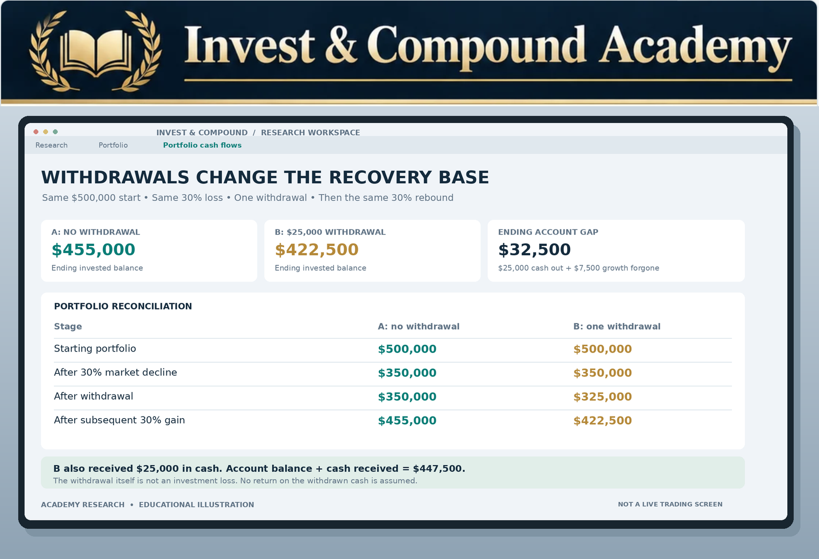
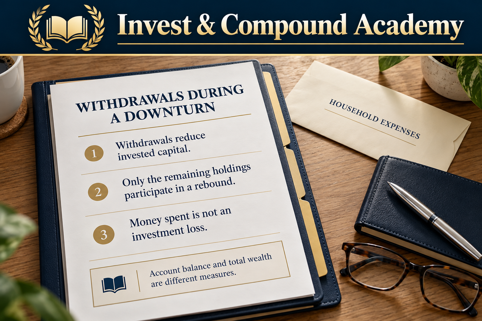
An investor already withdrawing money faces sequence-of-returns risk. Withdrawals during falling markets can reduce the number of shares remaining to participate in a recovery. This can make a prolonged downturn especially consequential.
Separate deposits, withdrawals and investment results with our guide to measuring investment growth. A recovering account balance and a recovering investment return are different measurements.
The Impact of Withdrawals During a Long Bear Market
Consider two hypothetical investors beginning with $500,000. Both experience the same market decline. Investor A does not withdraw funds during the downturn. Investor B makes one $25,000 withdrawal after the decline to cover living expenses. If both portfolios decline 30% before withdrawals, each falls to $350,000. Investor A retains the full $350,000 invested balance. Investor B withdraws $25,000, reducing the invested balance to $325,000. If both portfolios subsequently gain 30%, Investor A’s balance increases to $455,000. Investor B’s balance increases to $422,500.
The difference results from the withdrawal and the subsequent investment returns forgone on the withdrawn capital. Investor B also received $25,000 in cash. Adding that cash to the ending account gives $447,500, compared with Investor A’s $455,000. The $7,500 difference is the modeled growth forgone on the withdrawn money, assuming that cash earns no return. The $25,000 withdrawal itself is not an investment loss. The example models one withdrawal after the initial decline, not a recurring annual schedule.
It illustrates why recovery at the index level does not guarantee equivalent recovery for an investor making withdrawals.
Why Liquidity Reserves Matter
Cash and other liquid assets can help investors meet near-term expenses without selling volatile holdings. However, holding excessive cash for long periods creates opportunity costs and exposure to inflation. The appropriate reserve depends on spending needs, other income sources, household stability, and risk tolerance. The objective is to balance liquidity with long-term investment growth.
How Bear Markets Affect ETF Investors
Exchange-traded funds provide access to diversified portfolios and investment strategies. However, their performance during a bear market depends on their holdings. An ETF tracking the S&P 500 generally participates in broad U.S. equity-market movements. A technology-heavy ETF may experience a deeper decline when growth-oriented valuations fall. A dividend-oriented ETF can also suffer significant losses, even if distributions continue. Covered-call ETFs may receive option premiums that partially offset losses under certain conditions, but their distributions do not guarantee principal protection. Bond ETFs may provide diversification, although interest-rate changes and credit risk can also produce losses.
Why ETF Recovery Times Differ
An ETF’s recovery depends on the returns generated by its underlying assets. A broad equity index and a concentrated sector portfolio may recover at different speeds. Some sectors may regain previous highs quickly. Others may remain depressed after the broader market recovers. An investor should therefore avoid assuming that the historical duration of S&P 500 bear markets applies directly to every ETF.
Price Return Versus Total Return
Historical market studies frequently analyze price-index levels. An investor holding an ETF may receive cash distributions or reinvest those payments. Reinvested distributions affect total-return performance. Fund expenses and tracking differences also matter. For accurate comparisons, investors should understand whether historical results represent price returns, total returns, or actual fund performance.
Our dividend yield vs total return guide explains why cash distributions alone do not establish whether an investment has recovered.
Can Dollar-Cost Averaging Improve Outcomes During Long Bear Markets?
Dollar-cost averaging involves investing fixed amounts at predetermined intervals. This approach can be useful for investors who contribute regularly from earned income. When prices decline, the same contribution purchases more shares. When prices rise, it purchases fewer.
An Illustrative Example
Suppose an ETF initially trades at $100. An investor contributes $1,000 every month. Over four months, the ETF trades at $100, $80, $65, and $75. Ignoring fees and assuming fractional shares are available:
| Month | Share price | Contribution | Shares purchased |
|---|---|---|---|
| 1 | $100 | $1,000 | 10.0000 |
| 2 | $80 | $1,000 | 12.5000 |
| 3 | $65 | $1,000 | 15.3846 |
| 4 | $75 | $1,000 | 13.3333 |
The investor contributes $4,000. Approximately 51.218 shares are acquired. The average purchase cost is approximately $78.10 per share. At the final price of $75, the position remains below its total contribution value. If the ETF subsequently recovers, the additional shares purchased at lower prices can contribute to future gains. However, a prolonged decline or permanent impairment could produce continued losses. Dollar-cost averaging is therefore a disciplined contribution method, not a guarantee of investment success.
Should Investors Wait Until a Bear Market Ends Before Buying?
Waiting until a bear market has definitively ended may sound prudent. The difficulty is identifying that moment. A market can begin recovering before economic conditions improve visibly. It can also experience substantial temporary rallies before reaching a new low. Investors attempting to identify a precise bottom face uncertainty in both directions. Buying too early can expose capital to further losses. Waiting too long can mean missing part of the recovery.
Lump-Sum Investing
Deploying a lump sum immediately provides full market exposure. This can be favorable if markets subsequently rise. However, the entire amount is exposed if prices continue falling.
Gradual Investing
Deploying capital in stages reduces the amount exposed initially. It can make the process more manageable for investors uncomfortable with substantial short-term losses. However, gradual investment may underperform immediate investment when markets recover quickly.
The Appropriate Choice Depends on Circumstances
Neither method guarantees the best result. Relevant factors include investment horizon, available cash, risk tolerance, valuation, portfolio diversification, and financial obligations. The investor’s objective should be to make a decision consistent with an established strategy rather than rely on precise forecasting.
Why Bear-Market Rallies Complicate Timing
Bear markets do not necessarily involve uninterrupted declines. Strong rallies can occur during broader downturns. Investors may interpret those advances as evidence that the market has reached its final low. However, prices can subsequently decline again.
Short Covering
Investors who previously sold securities short may purchase shares to close positions. This buying can contribute to sharp upward movements.
Improved Expectations
Economic information may be less negative than investors anticipated. Markets can rally even when conditions remain unfavorable in absolute terms.
Policy Announcements
Central banks and governments may announce measures intended to support financial conditions. Such announcements can influence expectations and asset prices. However, policy responses do not guarantee that underlying economic problems have been resolved.
Valuation-Based Buying
Lower prices can attract investors seeking long-term opportunities. Yet valuation assessments differ, and new information can change the estimated value of an investment. For these reasons, a strong rally is not conclusive evidence that the bear market has ended.
How to Assess Bear-Market Risk Without Predicting the Bottom
A useful investment process focuses on resilience rather than exact market timing.
Evaluate Time Horizon
Capital needed for near-term obligations may not be suitable for substantial equity-market exposure. Longer horizons provide greater flexibility but do not guarantee positive returns.
Maintain Appropriate Liquidity
Accessible reserves can reduce the probability of forced selling during market weakness.
Review Concentration
A portfolio concentrated in one company, sector, or investment theme can suffer losses considerably greater than a diversified broad-market index.
Understand Leverage
Borrowing increases both potential gains and potential losses. Margin requirements can force asset sales during unfavorable market conditions.
Assess Investment Fundamentals
A decline in price does not automatically make an asset undervalued. Investors should consider business profitability, cash flows, debt obligations, and future prospects.
Establish Rebalancing Rules
A disciplined rebalancing policy can help maintain intended risk exposure. However, rebalancing does not guarantee profits or prevent additional losses. The purpose is portfolio alignment rather than prediction.
Use the ETF portfolio construction guide to connect allocation with your goals. For maintenance, see rebalancing ETFs with whole shares.
Can Diversification Shorten Portfolio Recovery Time?
Diversification may reduce concentration risk and moderate some portfolio drawdowns. However, it does not guarantee a shorter recovery period. The result depends on the assets held and their behavior during the relevant market environment. A portfolio combining equities and high-quality fixed income may experience smaller losses than an all-equity portfolio under certain conditions. In other environments, both asset classes can decline.
A Hypothetical Example
Consider two portfolios starting at $100,000. Portfolio A is invested entirely in equities. Portfolio B contains 60% equities and 40% bonds. Suppose equities fall 30% while bonds remain unchanged. Portfolio A declines to $70,000. Portfolio B’s equity allocation falls from $60,000 to $42,000, while its bond allocation remains at $40,000. Portfolio B is worth $82,000. The decline is 18%. Portfolio B requires approximately a 21.95% gain to recover, compared with approximately 42.86% for Portfolio A. This example demonstrates how a smaller drawdown can reduce the required recovery return.
However, it does not establish which portfolio will recover first. Future asset returns, correlations, and rebalancing decisions determine the actual outcome.
The Psychological Effect of Prolonged Bear Markets
Bear markets challenge more than financial calculations. They test an investor’s ability to tolerate uncertainty. A sudden decline can be frightening. A prolonged decline can be exhausting. Repeated losses, unsuccessful rallies, and uncertain economic forecasts may cause investors to question their original strategy.
Loss Aversion
Investors often experience losses more intensely than comparable gains. This can encourage decisions aimed at eliminating immediate discomfort. However, a decision made primarily to relieve anxiety may not align with long-term financial objectives.
Recency Bias
During extended downturns, investors may begin assuming that negative returns will continue indefinitely. This can lead to excessive pessimism. During strong bull markets, the opposite tendency can encourage investors to underestimate risk.
Overconfidence
Some investors become convinced that they can identify the exact market bottom. Others assume that a particular indicator guarantees further declines. Financial markets incorporate complex and changing information. No simple indicator has consistently identified every major turning point.
The Value of a Written Strategy
A written investment plan can establish target allocations, contribution policies, liquidity reserves, and circumstances that justify portfolio review. It does not eliminate uncertainty. It helps ensure that decisions are evaluated against financial objectives instead of changing emotional reactions.
Common Misconceptions About Bear-Market Duration
Every Bear Market Lasts About Ten Months
The historical average conceals substantial variation. Some declines reached their troughs within weeks, while others extended across hundreds of days.
Bear Markets End When Recessions End
Equity markets can begin recovering before a recession reaches its economic trough. The two timelines need not coincide.
A 20% Decline Means the Market Is Near the Bottom
The 20% threshold is descriptive. It does not establish a minimum price or indicate how much further markets may fall.
A Short Bear Market Always Produces a Fast Recovery
The duration of the decline and the recovery period are separate measurements. A short decline does not guarantee a short rebound.
Every Stock Eventually Regains Its Previous High
Individual businesses can suffer permanent capital impairment, bankruptcy, or prolonged competitive deterioration.
Investors Must Sell During Every Bear Market
The appropriate decision depends on liquidity, investment quality, financial objectives, and risk capacity.
Buying After a 20% Decline Guarantees Attractive Returns
Lower prices can improve investment opportunities, but future returns depend on valuation and underlying economic performance.
Diversification Eliminates Bear-Market Risk
Diversification can reduce certain risks but cannot eliminate broad equity-market declines.
Frequently Asked Questions
How Long Do Bear Markets Last on Average?
Hartford Funds’ historical analysis, based on Ned Davis Research data, reports an average peak-to-trough duration of approximately 289 calendar days across 27 bear-market episodes in the provider’s 1929–2024 table. The result depends on the methodology used to classify individual bear-market episodes.
How Many Months Does a Bear Market Usually Last?
The historical average above corresponds to approximately 9.6 months. However, the actual duration varies considerably. An average should not be used as a forecast.
What Was the Shortest Bear Market?
The 2020 pandemic bear market is among the shortest widely recognized S&P 500 bear markets in modern history. The Hartford Funds dataset records a 33-calendar-day decline from February 19 to March 23, 2020.
Can a Bear Market Last Several Years?
Yes. Broad downturns and the periods required to recover previous highs can extend for years. Some historical studies separate prolonged market collapses into multiple bear-market legs.
How Long Did the 2008 Bear Market Last?
The broader S&P 500 decline extended from its October 2007 peak to its March 2009 trough. Some datasets divide this period into separate bear-market segments. The duration therefore depends on the classification being used.
How Long Did the 2022 Bear Market Last?
Hartford Funds’ closing-price-based dataset records a decline lasting 282 calendar days between January 3 and October 12, 2022.
Does a Bear Market Always Mean a Recession?
No. Bear markets describe asset-price declines. Recessions describe contractions in economic activity. The two can overlap but do not always occur together.
How Long Does It Take to Recover From a 30% Market Loss?
A 30% decline requires approximately a 42.86% gain to return to the original value. The recovery period depends on subsequent investment returns and cannot be determined from the percentage loss alone.
Do Bear Markets Happen on a Fixed Schedule?
No. Historical averages describing frequency do not imply a predictable calendar cycle. Bear markets can occur close together or be separated by lengthy periods.
Do Dividends Help Investors Recover?
Dividends can contribute to total return, particularly when reinvested. However, payments are not guaranteed and do not eliminate market losses.
Should Investors Stop Retirement Contributions During Bear Markets?
There is no universal answer. Investors should consider income stability, liquidity, time horizon, allocation, and financial obligations. Regular contributions can acquire more shares at lower prices, but losses remain possible.
Are Bear Markets Good Times to Buy ETFs?
They can create opportunities when valuations become attractive. However, ETF prices may continue declining, and the underlying holdings may face fundamental challenges. Investment decisions should reflect individual circumstances.
Can Market Indicators Predict the End of a Bear Market?
No indicator consistently predicts every market bottom. Earnings expectations, credit conditions, valuations, and economic data can provide context but cannot establish a guaranteed recovery date.
Does a Market Recovery Mean the Economy Has Recovered?
Not necessarily. Stock prices reflect expectations about future economic and corporate conditions. Financial markets may recover before economic indicators show substantial improvement.
What Is the Most Important Lesson From Historical Bear Markets?
Bear-market duration is uncertain. Investors should build strategies that can withstand a range of adverse outcomes rather than depend on accurately predicting the next market bottom.
Bear Markets Have No Reliable Expiration Date
Historical data demonstrate that bear markets are recurring features of equity investing. Hartford Funds’ research reports an average peak-to-trough duration of approximately 289 days, but that figure summarizes a diverse collection of market environments. The 2020 pandemic decline reached its low within weeks. The 1973–1974 bear market continued for hundreds of days. The 2007–2009 financial crisis produced severe losses and a recovery process extending well beyond the decline itself. These episodes differed in their economic causes, monetary environments, financial-system conditions, and investor expectations.
Their common lesson is that bear-market duration cannot be predicted reliably using a simple historical average. Equally important, a market reaching its lowest point does not mean investors have fully recovered. The path back to a previous high depends on the depth of the decline and subsequent returns. For investors making withdrawals, the challenge may be even greater because capital removed during a downturn cannot participate in future recovery. A long investment horizon, suitable diversification, manageable leverage, adequate liquidity, and realistic return expectations can improve financial resilience. However, none eliminates the possibility of substantial losses.
A portfolio and financial plan should allow for unfavorable conditions to persist longer than anticipated. The useful planning question is whether your investment strategy can withstand a bear market that lasts longer than the historical average.
Continue Learning in the Invest & Compound Academy
Connect bear-market duration with the previous four market-risk pillars and practical portfolio planning.
Market risk, indexes and portfolio strategy
Market Correction Pillar | Indexes and Markets | Portfolio Construction
Sources and Further Reading
Reference review: October 18, 2026. Historical price declines use the cited provider’s cycle classification and calendar days. The historical table covers 1929–2024, with its last bear episode in 2022; source dated March 2025. Calculators and portfolio examples are hypothetical.
- Hartford Funds: Bear-Market History, based on Ned Davis Research
- NBER: U.S. Business Cycle Expansions and Contractions
- NBER: Business Cycle Dating Procedure
- Federal Reserve History: Stock Market Crash of 1929
- Federal Reserve History: Stock Market Crash of 1987
- S&P Dow Jones Indices: S&P 500 Overview
- SEC Investor.gov: Asset Allocation and Diversification
This article provides general education, not personalized investment, financial planning, legal or tax advice or a recommendation to buy, sell or hold a security.
Classification rules affect historical counts and durations. Past performance does not guarantee future results. Investments can lose principal permanently. The calculators simplify investment relationships and disclose their assumptions alongside the results. Consider your circumstances and consult qualified professionals where appropriate.