How Long Do Market Corrections Last? Duration and Recovery
Separate the decline from the rebound, compare historical episodes carefully, and understand why your portfolio’s recovery may follow a different timeline.
How long do market corrections last? When stock markets decline sharply, investors naturally want to know when the selling will stop and when their portfolios might recover. Watching an investment portfolio lose value creates uncertainty, particularly when the decline continues for several weeks and financial headlines offer conflicting explanations. Some analysts suggest that the market is approaching a bottom. Others warn that the decline could become a prolonged bear market. Meanwhile, investors must decide whether to maintain their investments, increase contributions, reduce exposure, or preserve cash.
Historical market statistics can provide useful perspective, but they do not offer a dependable countdown to recovery. Market corrections have lasted anywhere from relatively brief episodes to declines extending across several months. More severe downturns can continue substantially longer, especially when falling stock prices coincide with economic recessions, deteriorating corporate earnings, or financial-system stress. Fidelity’s April 2026 education article cites an average of about 115 days, attributed to Yardeni Research. Its summary does not fully spell out the sample and duration convention; that number should not be presented as a full-recovery deadline.
The estimate provides context, but it does not establish how long a current decline—or its subsequent recovery—will last. The distinction between the duration of the decline and the duration of the recovery is especially important. A market might reach its lowest level after three months but require another six months to regain its previous high. Another decline might happen in two weeks and recover almost immediately. A third might initially appear to be an ordinary correction, only to deepen into a bear market lasting substantially longer. For investors, understanding these possibilities is more useful than treating historical averages as forecasts.
This guide examines how market correction duration is measured, what historical evidence reveals, why recoveries differ, and how investors can evaluate the financial consequences of an uncertain recovery timeline. It also explores the role of valuations, monetary policy, earnings expectations, investor psychology, and portfolio construction in determining how vulnerable an investor may be to a prolonged period of market weakness.
How Long Does a Typical Market Correction Last?
Market corrections do not follow a standard timetable. A correction is commonly associated with a stock market decline of at least 10% from a recent peak. When classifying completed downturns, analysts typically distinguish corrections that remain below 20% from bear markets that reach or exceed 20%. The definition concerns the magnitude of the price decline, not its duration. A market can fall 10% in a single day. Another market might gradually decline 12% over four months. Both can meet the conventional numerical definition.
Fidelity’s historical estimate of approximately 115 days for a correction should be interpreted carefully because it depends on the dataset, observation period, and methodology of the underlying research. Some studies measure trading days, while others measure calendar days. Some use closing prices. Others use intraday highs and lows. Some include downturns that ultimately become bear markets, while others separate those episodes into different categories. As a result, there is no single universally applicable average.
Why the Average Is Not a Forecast
Suppose five hypothetical corrections last 18, 35, 60, 110, and 230 calendar days. Their average duration is:
Yet three of the five corrections last 60 days or less. The median duration is 60 days. The unusually long episode increases the arithmetic average. This example highlights a limitation of summary statistics. Financial market downturns have uneven distributions. A small number of particularly long episodes can influence the average substantially. Even a statistically accurate historical average does not establish how long the next correction will last. Markets are influenced by changing economic conditions, corporate earnings, monetary policy, liquidity, technology, and investor expectations. These factors do not repeat in identical combinations.
For that reason, investors should treat duration statistics as descriptive historical information rather than a scheduling tool.
For the definition and broader mechanics, start with our complete market-correction guide. This article focuses on measuring duration and planning for an uncertain recovery period.
Reference: Fidelity’s correction overview. Check the underlying dataset before comparing its average with other reported durations.
The Three Different Ways to Measure a Market Correction
When someone asks how long a market correction lasts, the answer depends on which period they want to measure. There are three important time intervals.
Peak-to-Trough Duration
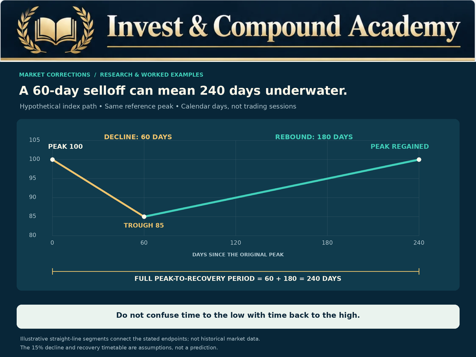
Peak-to-trough duration measures the time between the market’s previous high and its subsequent lowest point. Imagine an index reaches 5,000 on January 2. It gradually declines and reaches 4,250 on March 18. The index has fallen 15%. The peak-to-trough duration is approximately two and a half months. This measure describes the period during which the maximum decline developed. It does not indicate when the market returned to its previous high.
Trough-to-Recovery Duration
Trough-to-recovery duration begins at the market’s lowest point. It ends when the index regains its previous peak under the researcher’s specified methodology. Continuing the example, suppose the index reaches its low on March 18 and returns to 5,000 on September 20. The trough-to-recovery period is approximately six months. Investors experienced the deepest loss in March, but the recovery process continued for several additional months.
Peak-to-Recovery Duration
Peak-to-recovery duration combines the decline and recovery periods. In the same example, the index peaked in early January and regained its previous high in late September. The complete recovery period lasted approximately eight and a half months. For investors who hold through the entire episode, this period may be the most meaningful measure. It describes how long the market remained below the original peak.
Comparing the Three Measurements
| Measurement | Starting point | Ending point | What it explains |
|---|---|---|---|
| Peak-to-trough | Previous market high | Subsequent market low | Duration of the decline |
| Trough-to-recovery | Market low | Return to previous high | Duration of the rebound |
| Peak-to-recovery | Previous high | Return to that high | Complete underwater period |
These measurements are not interchangeable. An article reporting that a correction lasted 50 days may be describing only the decline. Another article reporting a six-month recovery may be describing the full peak-to-recovery period. Both figures may be accurate under their respective definitions. Investors should examine the methodology before comparing them.
Why the S&P 500 Is Commonly Used to Study Corrections
The S&P 500 is one of the most widely followed benchmarks for large U.S. equities. It provides a useful foundation for examining historical market drawdowns because of its broad coverage and extensive available data. However, the index does not represent every investment. The S&P 500 is weighted by float-adjusted market capitalization, meaning larger companies generally have greater influence on its performance. A decline in several heavily weighted companies can therefore produce substantial index-level weakness even when some smaller constituents remain relatively stable.
Conversely, individual stocks and industry sectors can experience major corrections without the S&P 500 itself reaching the 10% threshold.
Price Index Versus Total Return Index
Historical correction studies frequently use the price level of the S&P 500. A price index measures changes in the quoted index level without assuming that ordinary cash dividends are reinvested. A total-return index includes the effect of reinvested distributions according to the index provider’s methodology. This difference can affect recovery dates. An investor receiving and reinvesting dividends may experience a different total-return recovery timeline from an index measured using prices alone. Fund expenses, taxes, trading costs, and currency changes can create further differences in realized portfolio performance.
For consistency, comparisons of historical corrections should specify which return series is being used.
Calendar Days Versus Trading Days
Stock markets do not operate every calendar day. Weekends and market holidays create gaps between trading sessions. A decline lasting 40 trading days therefore covers more than 40 calendar days. When researchers compare duration statistics, they should avoid mixing the two units. A study reporting a 60-trading-day correction cannot be compared directly with one reporting 60 calendar days without adjusting the definitions. This distinction becomes especially important when evaluating relatively short downturns.
For the benchmark’s construction, see how the S&P 500 works.
How Often Do Market Corrections Occur?
The frequency of corrections provides context for their duration. If corrections are recurring market events, investors should expect meaningful drawdowns to appear periodically throughout long investment horizons. Fidelity’s March 2026 research found that from 1980 through 2025, the S&P 500 experienced an intrayear decline of at least 10% in 48% of calendar years. Over the same period, it recorded an average calendar-year total return of 13.3%. These findings demonstrate that significant temporary losses can coexist with positive long-term market performance. However, the statistics measure different things.
The 48% figure concerns the proportion of calendar years containing at least one qualifying intrayear decline. It does not identify the number of independent correction episodes. It also does not mean that investors should expect exactly one correction every two years.
Why Market Corrections Cluster
Financial-market volatility is not evenly distributed. Periods of economic uncertainty may produce repeated declines. Other periods feature sustained advances with relatively little interruption. Suppose an index experiences corrections in two consecutive years, followed by four years without a 10% decline. An investor interpreting the long-term average as a regular schedule would misunderstand how these events occur. Corrections are influenced by evolving conditions, not a fixed clock.
Why Long Periods Without Corrections Can Be Misleading
Extended market advances may encourage investors to believe that meaningful declines have become less likely. However, the absence of a recent correction does not prove that market risk has disappeared. Valuations may have increased. Corporate earnings expectations may have become more demanding. Investor positioning may have become concentrated. Nevertheless, none of these conditions guarantees that a correction is imminent. Markets can continue rising despite elevated valuations or growing economic concerns. The frequency of past corrections is therefore useful for setting expectations about volatility, not selecting a precise market entry or exit date.
Source: Fidelity’s March 2026 correction review, with calendar-year data through December 31, 2025. The annual-return figure includes dividends.
How Market Corrections Develop Over Time
Although every correction is different, the evolution of a downturn often reflects several interacting processes. Understanding these processes helps explain why some declines end relatively quickly while others continue.
Initial Market Repricing
A correction may begin when investors reassess the prices they are willing to pay for future corporate earnings. This can happen after an inflation surprise, a disappointing earnings report, an interest-rate announcement, or unexpected geopolitical developments. Initially, investors may believe the decline is temporary. Some market participants purchase shares because they consider the lower prices attractive. Others reduce exposure because they anticipate further deterioration. The competing expectations create volatility.
Increasing Uncertainty
As the decline continues, investors may begin questioning whether the original catalyst has broader consequences. A concern about interest rates may develop into concern about economic growth. A disappointing corporate earnings report may lead investors to reconsider expectations for an entire industry. A geopolitical disruption may affect commodity prices and corporate costs. This process can extend the correction because investors continuously update expectations as new information becomes available.
Selling Pressure and Positioning
Market prices also respond to trading behavior. Investors using leverage may face increasing collateral requirements. Some institutions may need to rebalance portfolios. Investment funds may experience withdrawals. Short-term trading strategies may respond to changes in volatility. These processes can contribute to temporary selling pressure even when underlying business fundamentals have not changed proportionately.
Stabilization
A correction may begin stabilizing when expectations stop deteriorating. Economic reports may improve. Corporate earnings may prove more resilient than feared. Financial conditions may become less restrictive. Lower valuations may attract long-term investors. However, stabilization is difficult to identify in real time. A market can experience a substantial rally and subsequently fall to a new low. The final trough becomes clear only retrospectively.
Why Some Corrections Recover Quickly
Several conditions can contribute to relatively rapid recoveries. The first is limited deterioration in corporate fundamentals. If businesses continue generating healthy earnings and cash flows, investors may conclude that previous selling was excessive. A second factor is improving clarity around the original catalyst. For example, a market decline driven by uncertainty about an anticipated policy decision may reverse when investors gain a clearer understanding of the likely outcome. A third factor is valuation. If prices fall while long-term earnings expectations remain relatively stable, prospective returns may become more attractive. Finally, liquidity and financial conditions matter.
Markets can recover more readily when investors retain access to financing, credit markets function normally, and forced selling diminishes. None of these conditions guarantees an immediate rebound. A market may remain weak even after fundamentals begin improving. Investor expectations and risk preferences can change slowly.
Why Other Corrections Last Much Longer
Longer corrections may reflect persistent uncertainty or changing economic conditions.
Continuing Inflation Pressure
Persistent inflation can affect corporate costs and household purchasing power. If central banks respond with restrictive monetary policy, borrowing costs may remain elevated. Investors may repeatedly revise valuations as expectations change. The correction can therefore extend beyond the initial inflation surprise.
Weakening Corporate Earnings
A decline in expected profits can require more than one adjustment to equity prices. Early in the downturn, analysts may still forecast relatively strong earnings. As new information emerges, forecasts may be reduced. Investors can respond with further repricing. If earnings expectations continue deteriorating, market recovery may be delayed.
Credit-Market Stress
When financing becomes more expensive or difficult to obtain, businesses may reduce investment and spending. Highly leveraged companies may face refinancing challenges. Financial institutions may become more cautious about lending. These developments can prolong economic weakness and increase uncertainty about future earnings.
Valuation Excesses
A market that begins with particularly elevated valuations may require a meaningful adjustment before investors view expected returns as attractive. However, valuation levels do not provide a reliable short-term timer. Markets can remain expensive or inexpensive for extended periods.
Economic Recession
A recession can create additional pressure on corporate profits and investor confidence. However, the relationship between recessions and market corrections is not mechanical. Some corrections occur without recessions. Markets can also begin recovering before recessions end because investors anticipate improving economic conditions.
A valuation multiple can change independently of earnings. See P/E ratio explained for the arithmetic behind that repricing.
What Historical Corrections Teach Us About Duration
Historical examples demonstrate the variability of market downturns. The four-episode comparison uses Shibui Finance’s published SPY ETF price history, updated October 12, 2026. It uses calendar days, closing prices without reinvested dividends, and recovery to the first close above the prior peak. SPY is a proxy, not the S&P 500 price index; their dates can differ. It is important to avoid combining correction episodes and bear markets without identifying the relevant classification.
The 1998 Market Decline
During 1998, emerging-market stress and concerns surrounding financial institutions contributed to substantial market volatility. The S&P 500 experienced a significant decline during the summer. The published SPY series reports an approximately 19% decline from July 17 to August 31, 1998. The peak-to-trough phase lasted approximately 45 calendar days. In that proxy series, the prior peak was regained on November 23. Under that dataset, the trough-to-recovery interval was approximately 84 days. This example illustrates how a correction approaching the bear-market threshold can still recover without evolving into a prolonged bear market on a closing-price basis.
It also illustrates a methodological complication: the episode briefly crossed the 20% threshold using some intraday measurements. The classification depends on whether closing or intraday prices are used.
The 2015–2016 Correction
Global growth concerns, commodity-market weakness, and uncertainty surrounding monetary policy contributed to substantial equity volatility during 2015 and early 2016. The same SPY series reports a roughly 14.4% decline from May 21, 2015, to February 11, 2016. The peak-to-trough period lasted 266 calendar days. Recovery to the previous high required another 152 days. This episode demonstrates that even a decline well below 20% can unfold over a prolonged period. It also shows why the depth of a correction does not determine its duration. A relatively moderate decline may involve repeated rallies and renewed weakness over several months.
The Early 2018 Correction
During early 2018, inflation concerns and changing interest-rate expectations contributed to increased market volatility. The S&P 500 experienced a decline exceeding 10% after reaching a January high. The SPY dataset identifies a January 26 peak and an April 2 trough; these are proxy closing-price dates, not an assertion about the price index’s lowest close. The peak-to-trough duration was 66 calendar days. In that series, recovery to the prior peak occurred on August 24. The trough-to-recovery period was approximately 144 days.
For investors, this illustrates the distinction between a decline that develops over roughly two months and a complete recovery that requires a substantially longer period.
The 2025 Correction
The 2025 U.S. equity decline provides a more recent example. Fidelity’s third-quarter 2025 investment research documented a particularly rapid decline of approximately 19.5% between February 19 and April 8, using its stated methodology. The peak-to-trough period was approximately 48 calendar days. Its research emphasized that the episode approached the conventional bear-market threshold very quickly. The SPY dataset reports about 19% and recovery on June 27, with an 80-calendar-day rebound.
Fidelity’s study analyzes weekly S&P 500 observations and rounds losses between 19.5% and 20% to 20% for its analysis. That is a different instrument and convention from the SPY table and from a strict closing-index classification. Investors should not assume that every report uses the same observations, rounding, or return series.
What These Episodes Demonstrate
The examples show that correction durations can differ dramatically. One significant decline took less than two months to reach its low. Another extended over most of a year. Recovery timelines also differed. No single historical episode provides a reliable model for the next correction. The underlying economic conditions, valuations, investor positioning, and financial environment all influence outcomes.
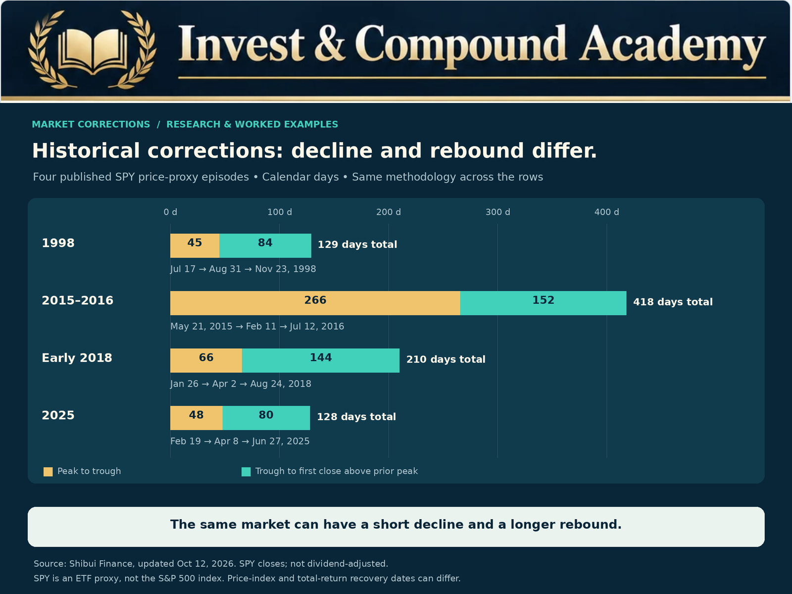
Historical proxy source: Shibui Finance’s SPY drawdown table and methodology. The separate near-bear-market comparison comes from Fidelity’s Q3 2025 research, page 4.
Why a Correction Can Become a Bear Market
A market decline initially classified as a correction may deepen beyond 20%. At that point, it enters conventional bear-market territory. The transition does not necessarily result from a new event. It may reflect continued deterioration in the same conditions that caused the original decline. Suppose an index peaks at 6,000 and falls to 5,280. The decline is 12%. Investors may initially expect a relatively short correction. If corporate earnings weaken and financial conditions tighten, the index may fall further to 4,650. The cumulative decline from the original peak is 22.5%. The episode has now crossed the bear-market threshold.
An investor who assumed that all corrections stop before 20% would have underestimated the potential downside.
The Problem With Treating 20% as a Protective Boundary
The market does not recognize the 20% threshold as a floor. A decline can continue well beyond it. The 2007–2009 global financial crisis and the 2020 pandemic collapse demonstrate that severe market episodes can cross the correction threshold rapidly and continue significantly lower. Consequently, historical averages for corrections that remain below 20% should not be applied uncritically to declines that are still unfolding. A current 12% drawdown may eventually be classified as part of a larger bear market. Its final classification is uncertain until the subsequent market path becomes clear.
Our market correction vs bear market comparison explains the classification boundary. The bear-market guide examines the liquidity, leverage and earnings pressures that can accompany deeper losses.
Does the Speed of a Decline Predict Its Recovery?
Investors often assume that a rapid decline should be followed by a rapid recovery. The argument is that sudden selling may create temporary mispricing, attracting buyers when uncertainty diminishes. Some historical episodes have followed this pattern. However, the relationship is not reliable enough to support a guaranteed investment rule. Fidelity’s 2025 sector research examined severe declines and found that faster drawdowns in its selected historical sample were frequently associated with strong subsequent twelve-month returns.
The study covers January 1957–May 2025 and measures next-twelve-month returns. A positive subsequent return does not necessarily mean the old peak was regained within those twelve months. The result depends on the sample, threshold, and observation period. It should not be treated as proof that every rapid decline will reverse quickly.
Why Recovery Speed Is Difficult to Predict
A rapid selloff caused by temporary liquidity pressure may reverse when buyers return. A similarly rapid decline caused by permanent deterioration in expected cash flows may require a very different adjustment. Markets may also experience several stages of repricing. An initial selloff can be followed by a rebound, additional negative news, and another decline. This sequence can make the final recovery timeline much longer than investors initially expect. The speed of the first decline is therefore only one piece of information. Investors should also evaluate the underlying catalyst, earnings expectations, financial conditions, and valuations.
Why Recovery to a Previous High Matters
Investors frequently evaluate losses in terms of their portfolios’ previous maximum values. This makes recovery to the former peak an intuitive benchmark. However, it is important to understand the mathematics. A 10% decline does not require a 10% rebound. A 15% decline does not require a 15% rebound. The percentage gain required to recover is larger because the calculation begins from a reduced capital base.
Recovery Mathematics
| Decline from peak | Value of a $10,000 investment | Required recovery |
|---|---|---|
| 10% | $9,000 | 11.11% |
| 12% | $8,800 | 13.64% |
| 15% | $8,500 | 17.65% |
| 18% | $8,200 | 21.95% |
| 20% | $8,000 | 25.00% |
| 25% | $7,500 | 33.33% |
| 30% | $7,000 | 42.86% |
These figures illustrate why a market’s recovery duration is influenced by the depth of its decline. A deeper decline requires a larger subsequent percentage gain. However, depth does not independently determine recovery time. Prices can rise rapidly under some conditions and recover slowly under others. A 25% decline followed by strong sustained gains could recover sooner than a 12% decline followed by years of weak performance.
The Difference Between Price Recovery and Investor Recovery
An index returning to its former high does not guarantee that every investor has recovered their losses. Individual outcomes depend on purchase timing, contributions, withdrawals, taxes, fees, and the assets held.
Investors Who Purchased at Different Prices
Suppose an ETF reaches $100, declines to $80, and later returns to $100. An investor who purchased at the original peak has recovered the initial price decline, excluding distributions and expenses. Someone who purchased at $90 during the decline has gained approximately 11.11% by the time the ETF returns to $100. An investor who purchased at $80 has gained 25%. The index recovery date is identical, but the investment outcomes differ.
Investors Who Continued Contributions
A person contributing regularly during the downturn may accumulate additional shares at lower prices. Those shares can participate in the subsequent recovery. The contribution adds capital as well as market exposure. Compare cash-flow-adjusted returns before concluding that the contribution decision improved investment performance; the result also depends on subsequent prices.
Investors Who Made Withdrawals
An investor withdrawing capital during the decline may not recover as quickly as the underlying index. Selling shares while prices are depressed reduces the number of shares remaining to participate in a rebound. This is particularly important for retirees and others who rely on investment portfolios for spending.
Currency Differences
International investors may measure returns in currencies different from the currency of the underlying index. For a Canadian investor holding U.S. equities without currency hedging, changes in the Canadian dollar relative to the U.S. dollar can affect returns measured in Canadian dollars. The U.S. index may regain its previous value while the Canadian-dollar value of the investment follows a different path. Currency movements can either amplify or offset underlying market returns.
An account balance can recover because new savings were added. Our guide to measuring investment growth separates those cash flows from the investment result.
How a Long Correction Affects Compound Growth
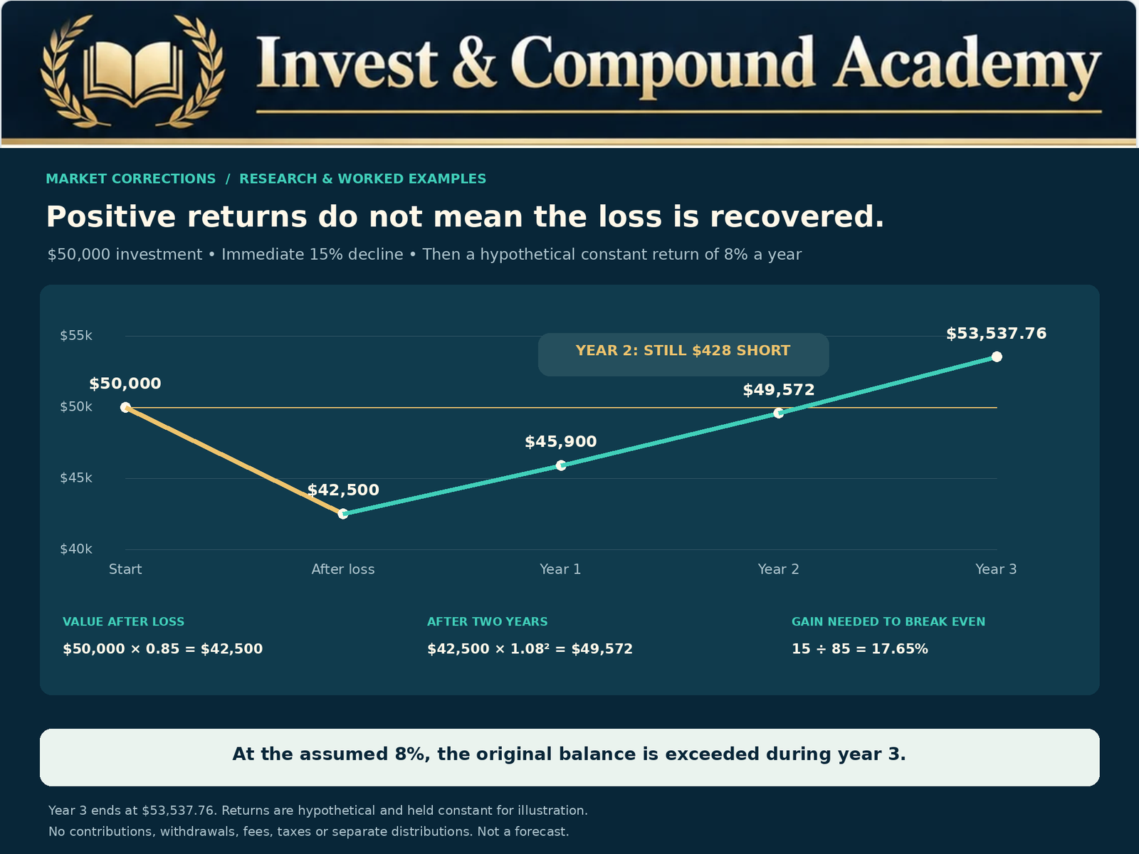
Compound growth depends on investment performance accumulating over time. Negative returns reduce the capital base available for subsequent growth. A prolonged correction can therefore delay progress toward a financial target. Consider a hypothetical investment beginning at $50,000. Assume it experiences a 15% decline. The balance falls to $42,500. If the portfolio subsequently gains 8% annually for two years, its value becomes:
Despite two consecutive years of positive returns, the investment remains slightly below its original $50,000. The example excludes distributions, fees, taxes, contributions, and withdrawals. It illustrates why recovering from losses can take time even after markets begin rising.
Volatility and Compound Returns
Suppose an investment gains 25% in one year and loses 20% in the next. Beginning with $10,000: After the first year, the portfolio is worth $12,500. After the second year, it returns to $10,000. The arithmetic average annual return is 2.5%. The compounded annual return over the two-year period is 0%. This demonstrates why average annual returns may not accurately describe the growth experienced by an investor. Volatility changes the capital base on which subsequent returns are earned. For long-term wealth-building strategies, compound returns and drawdown characteristics deserve attention alongside arithmetic averages.
How Corrections Affect Long-Term ETF Investors
Investors who hold broad-market ETFs may experience corrections without needing to change their long-term strategy. However, the appropriate response depends on the fund’s holdings, the investor’s financial position, and the original investment objective. An S&P 500 ETF can experience substantial interim losses while remaining diversified across many large U.S. companies. But diversification within equities does not eliminate overall market risk.
Broad Equity Exposure
A broad-market ETF reduces dependence on the financial condition of any one company. However, its value can still decline when investors reduce the valuations assigned to equities. The fund’s recovery depends on the performance of its underlying securities.
Sector Concentration
Technology-heavy or sector-specific ETFs may experience deeper drawdowns than broad-market indexes. Some sectors can remain weak even after the broader market recovers. Investors should not assume that every fund has the same correction duration.
Dividend-Oriented ETFs
Dividend-focused ETFs may generate recurring cash distributions during periods of market weakness. However, distributions do not guarantee positive total returns or prevent share-price declines. Dividend payments can also change. A fund’s quoted distribution yield should not be confused with its expected total investment performance.
Covered-Call ETFs
Covered-call strategies generate option premium income that may partially offset market losses. However, premium income does not establish a guaranteed protective floor. Certain strategies also limit participation in strong market advances. Investors should understand the relationship between distributions, underlying asset performance, option exposures, and total return.
The VOO vs QQQ comparison illustrates different index exposures. For income funds, read dividend yield vs total return before judging recovery from distributions alone.
Can Dollar-Cost Averaging Help During a Long Correction?
Dollar-cost averaging involves investing predetermined amounts at regular intervals. For investors contributing from ongoing income, the approach can reduce dependence on choosing a precise entry date. A fixed contribution purchases more shares when prices are lower. However, continuing contributions during a falling market does not guarantee gains.
Hypothetical Example
Suppose an investor contributes $500 each month to an ETF. Over four months, the ETF trades at $100, $90, $80, and $85. Ignoring fees and assuming fractional shares are permitted:
| Month | ETF price | Contribution | Shares purchased |
|---|---|---|---|
| 1 | $100 | $500 | 5.0000 |
| 2 | $90 | $500 | 5.5556 |
| 3 | $80 | $500 | 6.2500 |
| 4 | $85 | $500 | 5.8824 |
The investor contributes $2,000 and acquires approximately 22.688 shares. The average cost is approximately $88.15 per share. At the final price of $85, the position remains below its total purchase cost. If prices recover, the additional shares purchased at lower levels can contribute to future gains. But a prolonged decline could result in continued unrealized losses.
A Longer Correction Can Create Both Opportunity and Risk
A longer period of lower prices allows an investor making regular contributions to purchase more shares at reduced prices. That can be beneficial if the underlying investment eventually appreciates. However, the investor remains exposed to the risk of continued losses, permanent capital impairment, or a recovery taking longer than anticipated. Dollar-cost averaging is an investment process, not a guarantee against adverse outcomes. The strategy should be supported by sufficient liquidity, an appropriate asset allocation, and a realistic investment horizon.
What If You Need the Money Before the Market Recovers?
This question is often more important than the historical average duration of a correction. An investor may be financially capable of holding through a two-year recovery period but unable to wait if the capital is needed in six months.
Short-Term Financial Goals
Money intended for a near-term obligation may require more stable investment vehicles. Examples include a home down payment, tuition payment, business expense, or major planned purchase. If the timing of the obligation is inflexible, substantial equity-market exposure can create a mismatch between investment risk and spending needs.
Retirement Withdrawals
Retirees may need to finance living expenses during market downturns. Selling depressed investments can reduce the capital available for recovery. The resulting sequence-of-returns risk depends on the relationship between market performance and withdrawals. A strategy with adequate liquid reserves and a suitable asset allocation may provide greater flexibility.
Emergency Expenses
Unexpected financial needs can arise while markets are depressed. An investor who must liquidate equities to cover an emergency may be unable to wait for a recovery. Emergency reserves can reduce reliance on selling volatile investments at unfavorable times. The appropriate amount depends on household circumstances and income stability.
Why Market Timing Is Difficult During Corrections
Investors sometimes attempt to avoid a correction by selling equities and purchasing them again after prices decline. The approach appears attractive because successful execution could preserve capital and allow reinvestment at lower prices. However, it requires at least two successful decisions. The investor must identify a useful time to exit. Then the investor must identify an effective time to reenter. Both decisions occur under uncertainty.
Selling Too Early
An investor may sell because valuations appear high or economic indicators seem unfavorable. However, markets can continue rising for extended periods. The opportunity cost of remaining out of the market can become substantial.
Reentering Too Late
A market may recover quickly after the trough. Investors waiting for clear evidence that economic conditions have improved can miss part of the rebound. This is possible because financial markets incorporate expected future developments. Prices may begin rising while current economic reports remain disappointing.
False Recoveries
A market can rally during a correction and subsequently decline again. An investor interpreting every rally as the end of the downturn may make repeated transactions without improving the outcome.
Costs and Taxes
Frequent trading can generate transaction costs, spreads, and tax consequences. These factors can reduce returns even when the investor makes some successful timing decisions. For these reasons, the practical value of market timing cannot be evaluated solely by comparing ideal entry and exit prices known after the event.
Can Economic Indicators Tell Us When a Correction Will End?
Investors examine a wide range of indicators to assess market conditions. These include earnings revisions, inflation, interest rates, credit spreads, volatility, and market breadth. Each provides information about a different aspect of the financial system. None reliably identifies the exact date of a correction’s end.
Corporate Earnings
Improving earnings expectations may support equity valuations. However, stock prices can begin recovering before analysts revise their forecasts upward. Conversely, strong earnings reports may fail to lift prices if investors expected even better results.
Inflation
Moderating inflation may reduce concerns about monetary tightening. However, falling inflation can occur alongside weakening economic demand. Investors must evaluate the broader economic context.
Interest Rates
Lower expected interest rates may improve valuations under some circumstances. But rates can fall because economic conditions are deteriorating. The cause of the change matters.
Credit Spreads
Narrowing credit spreads may indicate improving investor confidence and financing conditions. However, credit spreads can respond quickly to market expectations and do not provide a guaranteed equity-market forecast.
Market Breadth
Improving participation across stocks may suggest that an advance is becoming more broadly supported. Nevertheless, breadth indicators can produce misleading signals. A market may remain concentrated for extended periods before experiencing meaningful weakness.
Volatility
Market volatility often rises during corrections. A subsequent decline in volatility may suggest that uncertainty is easing. However, volatility can remain elevated after the market begins recovering or temporarily decline before another selloff. The most useful role of these indicators is assessing economic and financial conditions, not constructing a precise recovery countdown.
How to Evaluate Your Portfolio During a Correction
A correction provides an opportunity to assess the relationship between portfolio risk and financial objectives. The objective should not be to react mechanically to the market’s percentage decline. Instead, investors can examine whether their portfolio remains appropriate.
Review the Investment Horizon
Capital required in the near future may not have sufficient time to withstand a prolonged recovery. An investor saving for retirement several decades away may have more flexibility. However, time horizon alone does not eliminate investment risk.
Evaluate Liquidity
Cash reserves and other accessible assets can reduce the likelihood of forced sales. Investors should consider employment stability, household obligations, debt payments, and foreseeable expenses.
Examine Concentration
A portfolio holding several ETFs may still be concentrated in a small group of companies or sectors. Underlying holdings and correlations matter more than the number of fund names.
Review Leverage
Borrowing against investments can create additional vulnerability. A market decline may cause collateral values to fall, potentially triggering margin calls or forced liquidation. Leverage can prevent investors from maintaining positions through a recovery.
Assess the Investment Thesis
A broad market correction does not automatically mean every company’s fundamentals have deteriorated. However, a decline can reveal weaknesses in particular businesses. Investors should consider profitability, debt obligations, competitive position, and expected cash generation.
Consider Rebalancing
Rebalancing can restore a portfolio toward its intended allocation. This may involve purchasing assets whose weights have fallen or reducing exposures that have become too large. However, rebalancing does not guarantee improved returns. Its primary purpose is maintaining the desired risk profile.
Connect risk to the goal with our ETF portfolio construction guide. The VOO and VTI overlap workbook helps identify shared holdings, while whole-share ETF rebalancing covers trade sizing and rounding.
The Psychological Challenge of Waiting for Recovery
Market corrections can be difficult because investors rarely know how much longer uncertainty will continue. A decline lasting two weeks may feel manageable. The same portfolio loss extending over six months can become more emotionally exhausting. Repeated rallies and reversals may increase frustration. Investors may begin questioning their strategy even when their financial objectives remain unchanged.
Recency Bias
Investors tend to assign considerable importance to recent events. During prolonged market weakness, they may begin expecting further losses indefinitely. During strong markets, they may underestimate the probability of a correction. Neither assumption provides a reliable foundation for investment decisions.
Loss Aversion
Financial losses can create strong emotional reactions. An investor may be tempted to sell simply to eliminate the discomfort of watching prices fluctuate. That decision may or may not be financially appropriate. The relevant consideration is whether the portfolio still fits the investor’s circumstances and investment thesis.
Information Overload
Modern investors have continuous access to market prices, commentary, forecasts, and economic data. Frequent exposure to financial headlines can create the impression that every development requires an immediate portfolio decision. A long-term investment plan can help distinguish meaningful changes from ordinary market noise.
The Value of a Written Plan
A documented investment process may establish target allocations, contribution schedules, liquidity reserves, and review intervals. The purpose is to provide consistency during uncertainty. It should remain adaptable when financial circumstances or fundamental assumptions genuinely change.
What Investors Should Avoid Assuming About Recovery
Several common beliefs can lead to poor decisions.
Every Correction Recovers Within Four Months
Historical averages do not guarantee a recovery date. Some corrections last considerably longer. Others evolve into bear markets.
A 10% Decline Means the Bottom Is Near
The 10% threshold is descriptive. It does not establish a support level or imply that selling pressure must end.
The Market Will Recover as Soon as Inflation Falls
Inflation is only one factor influencing equity valuations. Earnings, interest rates, credit conditions, and investor expectations also matter.
A Market Rally Means the Correction Has Ended
Temporary rallies can occur within broader declines. The market may subsequently reach a new low.
Every Individual Stock Will Recover
Broad market indexes have historically recovered from many downturns. Individual companies can experience permanent losses, bankruptcy, or sustained deterioration in profitability.
Investors Must Trade Frequently During Corrections
Frequent activity is not necessarily better risk management. For some investors, maintaining an appropriate allocation and continuing a disciplined contribution schedule may be consistent with their objectives. Others may need to adjust positions because of liquidity requirements, concentration, or changing fundamentals. The decision depends on individual circumstances.
Frequently Asked Questions
How Long Do Market Corrections Last on Average?
Fidelity’s April 2026 investor education cites a historical average of approximately 115 days from Yardeni Research. This is a descriptive estimate, not a prediction. Actual correction durations vary significantly, and the estimate should not be treated as a full-recovery deadline.
Can a Market Correction Last Only One Day?
A sufficiently sharp one-day decline can meet the conventional 10% threshold. However, the subsequent recovery may take longer.
Can a Correction Last More Than One Year?
A market may remain below a previous high for more than a year, and some declines can extend across long periods. Whether a particular episode is classified as a correction or bear market depends on the depth of the decline and the research methodology.
Does a Correction End When Stocks Rise 10% From the Low?
Not under every methodology. A 10% rebound from the trough does not necessarily restore the previous market high. Researchers may use different definitions for identifying the end of an episode.
What Is the Difference Between Correction Duration and Recovery Time?
Correction duration commonly refers to the period from peak to trough. Recovery time may refer to the rebound from trough to previous peak or to the entire peak-to-recovery interval. The measurement must be specified.
Do S&P 500 Corrections Recover Faster Than Individual Stocks?
There is no universal rule. Individual stocks can recover quickly, remain depressed for years, or fail permanently. A diversified index follows a different composition and risk profile.
Do Market Corrections Always Lead to Recessions?
No. Corrections can occur while the economy continues expanding. Market declines and economic recessions are related but distinct phenomena.
Should Investors Wait for a Correction to End Before Buying?
There is no strategy that guarantees the best outcome. Waiting may reduce exposure to additional immediate losses, but it may also cause investors to miss part of a recovery. Decisions should reflect valuation, liquidity, risk tolerance, and investment objectives.
Does Dollar-Cost Averaging Work Better During Long Corrections?
Regular contributions can accumulate more shares when prices remain lower. However, the strategy does not guarantee superior returns or protection against losses. Its outcome depends on subsequent investment performance.
Can Dividends Shorten an Investor’s Recovery Period?
Reinvested dividends can affect total-return performance. A total-return investment may regain its previous economic value at a different time from a price-only index. However, distributions are not guaranteed and do not prevent capital losses.
Can a Correction End Without Strong Economic Growth?
Yes. Financial markets respond to expectations about future conditions. Prices can recover when outcomes become less unfavorable than investors previously anticipated.
What Is the Most Important Factor for Investors During a Long Correction?
There is no single factor for everyone. Time horizon, liquidity, allocation, leverage, investment quality, and the need for withdrawals can all determine whether an investor can withstand an extended downturn.
Market Recovery Has No Reliable Countdown
The question of how long a market correction lasts has no single dependable answer. Historical research provides valuable perspective. Corrections have frequently resolved without developing into severe bear markets, and broad U.S. equities have recovered from many significant declines. But recovery timelines vary. Some corrections reach their lowest point in a matter of weeks. Others continue for many months. The period required to regain a previous high may be substantially longer than the decline itself.
Investors should therefore distinguish between three questions: how far prices have fallen, how long they have been falling, and how much time may be required to recover. Each describes a different dimension of investment risk. Historical averages can help investors understand the range of past experiences, but they cannot establish the next market bottom or recovery date. The more productive approach is to build a portfolio that does not depend on predicting those events accurately. Appropriate diversification, sufficient liquidity, realistic investment horizons, manageable leverage, and disciplined decision-making can improve financial resilience.
For long-term investors, the central issue is not whether every market correction can be avoided. It is whether the financial plan can withstand the uncertainty that accompanies one. Market history is valuable because it shows what has happened under different circumstances. It is not a calendar that tells investors exactly what will happen next. A resilient investment strategy allows for recovery to take longer than expected.
Continue Learning in the Invest & Compound Academy
Follow the market-risk series and connect recovery timelines with portfolio measurement and maintenance.
Market risk, indexes and portfolio strategy
Market Correction Pillar | Indexes and Markets | Portfolio Construction
Sources and Further Reading
Reference review: October 17, 2026. Source observation periods differ. The historical illustration uses the cited SPY proxy series; the other two illustrations are hypothetical. Examples are not live market measurements.
- Fidelity: What Is a Market Correction?
- Fidelity: A Game Plan for Market Corrections
- Fidelity: Quarterly Sector and Investment Research Update, Q3 2025, page 4
- Shibui Finance: SPY Drawdown History and Methodology—updated October 12, 2026
- S&P Dow Jones Indices: S&P 500 Overview
- SEC Investor.gov: Asset Allocation and Diversification
This guide provides general financial education, not personalized investment, tax or legal advice or a recommendation to buy or sell a security.
Historical averages do not predict recovery dates. Investments may lose value permanently. Calculators and numerical scenarios simplify financial relationships; their assumptions and exclusions are stated alongside them. Consider your circumstances and consult qualified professionals where appropriate.