Biggest Market Corrections in Stock Market History
Compare selected S&P 500 drawdowns, the pressures associated with them, and the recovery mathematics. Understand why similar losses can conceal very different economic risks.
The biggest market corrections show how different shocks can produce similar headline losses. Financial markets have experienced extraordinary changes throughout modern economic history. Wars, inflationary shocks, banking crises, technological revolutions, interest-rate changes, and unexpected geopolitical developments have repeatedly altered investor expectations and asset valuations. Some events produced relatively modest declines. Others triggered severe bear markets that erased substantial portions of accumulated wealth. Between those extremes lies a particularly important category of market volatility: the stock market correction.
A market correction is generally defined as a decline of at least 10% but less than 20% from a relevant previous market peak. Although the threshold is familiar, the historical circumstances behind individual corrections differ considerably. A decline can emerge because investors become concerned about inflation. Another may develop from problems in international credit markets. A third can follow changes in trade policy or uncertainty about future corporate earnings. The speed, severity, and eventual recovery of these episodes also vary.
Some of the largest corrections have approached the 20% bear-market threshold without crossing it under closing-price measurement. Others began as apparently ordinary corrections before deteriorating into much deeper downturns. The difference matters. A market that loses 19% and subsequently recovers provides a different historical example from one that declines 19%, continues falling, and eventually loses half its value. The initial losses may look similar, but the financial outcomes are not.
For investors, studying historical market corrections offers several benefits. It helps place market declines within a longer historical perspective, reveals how different economic shocks affect asset prices, and demonstrates why market recovery cannot be predicted using a single historical average. It also challenges several common assumptions. Corrections do not necessarily indicate an approaching recession. Deep market declines do not always require prolonged economic weakness. Rapid selling does not automatically produce rapid recovery, and a lower share price does not guarantee that an investment has become undervalued.
This guide examines major historical S&P 500 correction episodes, the financial conditions that produced them, and what their outcomes reveal about market behavior. It also distinguishes corrections from bear markets, explains the limitations of historical data, and translates the evidence into practical lessons about portfolio construction, diversification, liquidity, valuations, and investment discipline. The objective is not to predict the next correction. It is to understand the financial mechanisms that have shaped previous downturns—and how those lessons can improve the quality of future investment decisions.
What Qualifies as a Major Market Correction?
A market correction refers to a decline of at least 10% from a previous high. When describing a completed drawdown episode, analysts generally classify losses that remain below 20% as corrections. Declines reaching or exceeding 20% are conventionally described as bear markets. A decline of 19.5% is therefore a particularly severe correction under a methodology using that measurement. A decline of 20.5% crosses the bear-market threshold. However, the 20% boundary is a classification convention rather than a fundamental economic dividing line.
A market experiencing a 19.5% drawdown may face economic risks similar to one that has declined 20.5%.
Why Closing Prices Matter
Historical correction rankings depend on whether researchers use daily closing prices or intraday market levels. The distinction can change how an episode is classified. For example, a market might briefly trade 21% below its previous high during a particularly volatile session but finish the day only 19% below the reference peak. Using intraday data, the market crossed the conventional bear-market threshold. Using closing prices, it remained in correction territory. Neither measure is inherently meaningless. However, comparisons become unreliable when different measurement conventions are mixed without explanation.
The main comparison uses S&P 500 U.S.-dollar price-index closes. Drawdown is calculated as (trough close ÷ reference peak close − 1) × 100. Dividends, fees, taxes and currency translation are excluded. A completed episode is assessed after the fact; a 10% decline observed in real time can still deepen. Figures from different historical sources are identified as such and should not be interpreted as measurements obtained through one identical methodology.
Price Decline Versus Total Return
A price index measures changes in index levels without including the reinvestment of ordinary cash dividends. A total-return index accounts for reinvested distributions according to the index provider’s methodology. Over extended periods, the difference can be significant. An investor holding an index-tracking ETF with distributions reinvested may experience a different cumulative return and recovery date from the corresponding price index. Therefore, the historical correction figures discussed here should not automatically be interpreted as exact investment returns for every ETF shareholder. Actual results depend on the fund, expenses, distributions, purchase dates, taxes, and other factors.
For the broader definitions, read what a market correction means and our market correction vs bear market comparison. This article concentrates on historical episodes and their associated pressures.

Biggest Market Corrections: Selected S&P 500 Episodes
Several historical episodes demonstrate how close a market can come to the conventional bear-market threshold without clearly crossing it on a closing-price basis. The following table presents selected closing-price episodes. It is not an exhaustive ranking. Historical providers sometimes reset the reference peak after a substantial rebound rather than waiting for a new all-time high. The 2002–2003 recovery-period decline is identified separately for that reason.
| Historical episode | Approximate S&P 500 decline | Primary market concerns |
|---|---|---|
| 1989–1990 | 10.2% | Monetary conditions and economic uncertainty |
| 1990 | 19.9% | Gulf crisis, oil prices, and recession concerns |
| 1997 | 10.8% | Asian financial-market instability |
| 1998 | 19.3% | Emerging-market crisis and financial contagion |
| 1999 | 12.1% | Interest rates and equity valuations |
| 2002–2003 recovery-period correction | 14.7% | Economic uncertainty after the technology collapse |
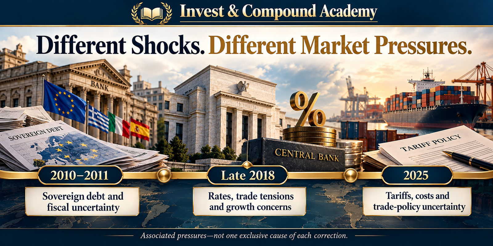
| 2010 | 16.0% | European sovereign debt and financial stability |
| 2011 | 19.4% | U.S. debt downgrade and European sovereign debt |
| 2015–2016, combined window | 14.16% | China, commodities, and global growth |
| Early 2018 | Approximately 10.2% | Inflation and interest-rate expectations |
| Late 2018 | Approximately 19.8% | Monetary tightening, trade tensions, and growth concerns |
| 2023 | Approximately 10.3% | Higher bond yields and restrictive rates |
| 2025 | Approximately 18.9% | Tariff announcements and trade-policy uncertainty |
Most rounded magnitudes are reported in First Trust’s Bloomberg-based table, dated March 28, 2024. That source includes bear-market legs as well as corrections; only the identified examples are selected here. The combined 2015–2016 window uses 2,130.82 on May 21, 2015 and 1,829.08 on February 11, 2016. The 2025 window uses 6,144.15 on February 19 and 4,982.77 on April 8. These are price-index measurements, not dividend-reinvested ETF returns.
The data reveal that significant declines can occur in very different environments. Some episodes followed international financial crises. Others were associated with domestic interest-rate expectations. Several occurred while the U.S. economy continued expanding. These differences demonstrate why the severity of a correction cannot be explained through a single economic variable.
The S&P 500 index guide explains what the benchmark measures. A local-peak drawdown and an uninterrupted decline from an all-time high can produce different episode counts.
Source notes: First Trust’s 2024 resource kit, final page; the Credit Suisse pricing supplement hosted by the SEC, historical Bloomberg closing-level table; and S&P DJI closing prices via FRED. SEC hosting does not imply verification or endorsement of the issuer’s figures.
The 1990 Correction: Oil Prices, Geopolitical Risk, and Recession
The 1990 market decline is one of the clearest examples of a correction approaching the conventional bear-market threshold. The S&P 500 experienced a peak-to-trough decline of approximately 19.9%, according to historical correction data cited by First Trust and other market researchers. The episode developed during a period of rising economic uncertainty. Iraq’s invasion of Kuwait in August 1990 created concerns about energy supplies and geopolitical stability. Oil prices increased sharply. Higher energy costs threatened consumer purchasing power and corporate operating expenses. At the same time, the U.S. economy was entering a recession.
The Economic Background
An increase in energy prices can influence the economy through several channels. Consumers may spend more on gasoline, heating, and transportation. Businesses face higher input costs. Companies with limited pricing power may experience pressure on profit margins. Investors may respond by revising earnings expectations downward. However, energy prices were not the only factor affecting the 1990 economy. Credit conditions, financial-sector problems, and broader economic weakness also contributed to the unfavorable environment.
Why the Market Declined
Investors faced uncertainty about both economic growth and inflation. Higher energy costs could weaken demand while placing upward pressure on prices. That combination made the outlook more difficult to assess. Stock valuations adjusted as expectations changed. The S&P 500 decline approached 20% without conclusively crossing that threshold under the cited closing-price methodology.
The Recovery Lesson
The episode illustrates why a severe correction can occur alongside a recession. It also shows that geopolitical shocks can amplify financial uncertainty without necessarily producing a prolonged multi-year equity collapse. Investors should not assume that every international conflict produces the same financial consequences. The effects depend on energy markets, economic conditions, policy responses, and investor expectations.
The 1997 Asian Financial Crisis: A Global Shock With Uneven Effects
The Asian financial crisis began as financial pressures intensified in several rapidly growing Asian economies. Currency instability, external debt obligations, and fragile financial systems created widespread uncertainty. The crisis affected regional currencies, banks, businesses, and capital flows. U.S. equities also experienced volatility. Historical S&P 500 correction data identify a decline of approximately 10.8% during October 1997.
Why Currency Crises Affect Stocks
Companies and financial institutions may borrow in foreign currencies. If a local currency falls sharply, the domestic-currency cost of repaying foreign-currency debt can increase. Businesses may struggle to meet obligations. Financial institutions can face losses. International investors may withdraw capital, placing further pressure on asset prices. These mechanisms can create a feedback loop.
Why the U.S. Market Was Affected
Although the crisis originated outside the United States, financial markets are globally connected. U.S. companies may depend on overseas demand, supply chains, and financing relationships. Changes in global risk appetite can also affect equity valuations. Investors sometimes reduce exposure across multiple markets during periods of uncertainty. Consequently, an economic disruption concentrated in one region can influence prices elsewhere.
Why the Decline Remained a Correction
The broader U.S. economic environment differed from the conditions in the most affected Asian countries. The U.S. market subsequently recovered without experiencing an equivalent domestic financial collapse. This demonstrates that market contagion does not necessarily imply identical economic outcomes. The severity of the effect depends on the exposure of individual companies, financial institutions, and economies.
Investor Lesson
International developments matter even for portfolios invested primarily in U.S. equities. However, the geographic origin of a crisis does not determine the extent of its ultimate impact on every market. Investors need to analyze actual economic exposures rather than assume that all global shocks produce the same losses.
The 1998 Correction: Russia, Emerging Markets, and Financial Contagion
The 1998 stock market correction was among the deepest U.S. market declines that remained below 20% under widely cited closing-price measurements. First Trust’s historical analysis reports an S&P 500 decline of approximately 19.34% from its relevant peak to the August 31, 1998, trough. The episode was associated with emerging-market financial instability, Russia’s debt crisis, and concern about highly leveraged financial institutions.
The Russian Debt Crisis
In August 1998, Russia announced measures involving its domestic debt and exchange-rate arrangements amid severe financial pressure. Investor confidence deteriorated. Concerns about sovereign debt, currency exposures, and counterparty risk spread through international financial markets. Emerging-market assets experienced substantial pressure.
The Role of Leverage
The episode also highlighted the risks associated with highly leveraged investment strategies. Long-Term Capital Management, a major hedge fund, experienced severe losses as market relationships changed and liquidity deteriorated. Its private-sector recapitalization occurred on September 23, 1998, after the August 31 S&P 500 trough cited here. It illustrates the wider financial-stress episode, rather than an event that preceded every part of the July–August decline. Positions that appeared relatively stable under ordinary conditions became difficult to maintain. Financial counterparties faced uncertainty about potential exposures.
Why Liquidity Became Important
During periods of financial stress, investors often seek to reduce risk quickly. But the ability to sell assets depends on available buyers. When many market participants attempt to sell similar positions simultaneously, liquidity can weaken. This may produce price changes larger than those explained by immediate revisions to long-term cash flows. The 1998 episode demonstrated how financing, leverage, and market liquidity can amplify financial uncertainty.
Recovery and Broader Implications
The S&P 500 subsequently recovered its previous closing high later in 1998. However, the rapid market recovery should not obscure the seriousness of the underlying financial stress. The episode helped demonstrate the potential systemic consequences of concentrated leveraged positions. For individual investors, the principal lesson concerns the difference between temporary market-price volatility and the financial consequences of being unable to maintain a position. An unleveraged investor with adequate liquidity may have options unavailable to an institution facing margin or collateral demands.

The 1999 Correction: Interest Rates and High Equity Valuations
During 1999, U.S. equity markets experienced a significant correction amid changing interest-rate expectations and growing concerns about valuation levels. Fidelity’s historical table identifies a correction beginning in July 1999 and reaching its trough approximately 91 days later. Other historical research estimates the decline at approximately 12.1%.
The Market Environment
The late 1990s were characterized by strong interest in technology and internet-related companies. Expectations for future growth became increasingly optimistic. Some companies were valued using assumptions that required exceptional future profitability. At the same time, monetary policy and interest-rate expectations influenced the relative attractiveness of stocks and bonds.
Why Higher Rates Matter
Higher interest rates can increase the required return investors demand from equities. When a larger discount rate is applied to future corporate cash flows, estimated present values generally decline, all else being equal. Companies whose valuations depend heavily on profits expected many years into the future can be particularly sensitive.
Why the Correction Did Not Resolve Every Valuation Risk
Although the 1999 correction eventually ended, many equity valuations remained demanding. The following years brought the much more severe technology-related bear market. This is an important historical distinction. A correction ending does not guarantee that every underlying valuation imbalance has disappeared. Short-term market recovery and long-term investment attractiveness are separate questions.
Investor Lesson
Markets can recover from a correction even while longer-term vulnerabilities remain. Investors should avoid assuming that the latest price rebound validates every previous valuation. Company fundamentals, cash-flow expectations, and the purchase price remain essential.
Our P/E ratio guide explains why a share-price rebound alone does not establish that earnings expectations or valuation assumptions are reasonable.
The 2002–2003 Correction: Volatility During a Market Transition
The period following the technology bubble illustrates how substantial market declines can occur during an attempted recovery from a previous bear market. Fidelity’s historical analysis identifies a correction beginning in November 2002. First Trust’s published statistics report a decline of approximately 14.7% to March 11, 2003. The market was still absorbing the economic and financial consequences of the technology downturn.
The Importance of Market Context
A correction following a severe bear market can differ from one occurring after a long expansion. Investors may be reassessing whether corporate earnings have stabilized. Previously overvalued industries may continue experiencing weakness. Financial confidence may remain fragile. Even as market prices recover from earlier lows, uncertainty can produce renewed selling.
Why Recovery Is Not Always Smooth
A market can experience several significant rallies and declines before establishing a durable advance. These movements do not necessarily represent independent economic crises. They may reflect changing expectations within a broader market transition.
Investor Lesson
Investors should distinguish between a market recovering from a major bear-market collapse and one experiencing a correction during a mature bull market. The historical background influences valuations, sentiment, and economic risks. Percentage declines alone do not provide sufficient context.
The 2010 Correction: European Sovereign Debt Concerns
The 2010 market correction was driven partly by concerns about sovereign debt sustainability and financial stability in Europe. The S&P 500 declined approximately 16% between its April peak and early July trough under a commonly cited closing-price measurement. The episode occurred during the recovery from the global financial crisis.
Why Sovereign Debt Became a Concern
Governments borrow to finance expenditures and refinance existing obligations. When investors become concerned about a government’s fiscal capacity, borrowing costs can rise. Higher yields increase financing pressure. In countries whose banks hold substantial amounts of sovereign debt, concerns about public finances can affect the banking system.
The Bank-Sovereign Relationship
Financial institutions frequently hold government securities. A decline in the value of those holdings can weaken balance sheets. At the same time, governments may face pressure to support domestic banks. This creates a potentially difficult relationship between sovereign risk and banking risk.
Why U.S. Equities Responded
Financial-market uncertainty in Europe affected expectations about global growth, credit conditions, and international financial stability. U.S. equities experienced significant selling pressure. However, the U.S. economy was not experiencing a repeat of the same financial conditions that characterized the 2007–2009 crisis.
The Recovery Lesson
The 2010 correction demonstrates that a serious international financial challenge can contribute to meaningful U.S. equity losses without automatically producing another global bear market. Investors should evaluate the channels through which international risks affect corporate earnings, credit, and economic activity.
The 2011 Correction: Debt Downgrade and European Financial Stress
The 2011 correction was another exceptionally deep episode. First Trust’s historical data report an S&P 500 decline of approximately 19.39%, with the market reaching a trough on October 3, 2011. The downturn was associated with several developments, including concerns about European sovereign debt, U.S. fiscal policy uncertainty, and the downgrade of the United States’ long-term sovereign credit rating by Standard & Poor’s.
The U.S. Debt-Ceiling Dispute
Political disagreements concerning federal borrowing authority generated uncertainty about fiscal management and financial obligations. Investors became concerned about the possibility of payment disruptions and broader effects on financial confidence.
The Credit-Rating Downgrade
In August 2011, Standard & Poor’s downgraded the United States’ long-term sovereign credit rating from AAA to AA+. The announcement attracted considerable attention. However, the market response reflected multiple overlapping concerns rather than a single announcement alone.
European Debt Concerns
Financial pressures in parts of Europe continued affecting investor expectations. Banks, government bond markets, and economic growth remained important sources of uncertainty. The combination of U.S. and European concerns contributed to heightened volatility.
Why the Correction Was Significant
The approximately 19.4% decline brought the market very close to the conventional bear-market threshold. Investors attempting to predict whether the downturn would stop before 20% faced substantial uncertainty. Small changes in market prices could have changed the classification.
Recovery and Lessons
The S&P 500 eventually recovered without the downturn becoming an extended bear market under the cited closing-price convention. The episode demonstrates why market classification should not substitute for understanding economic risk. A decline of 19.4% can have serious consequences for investors with concentrated positions, leverage, or near-term spending needs.
The 2015–2016 Correction: China, Commodities, and Global Growth
The 2015–2016 correction developed over an extended period of uncertainty. Measured from the May 21, 2015 closing high of 2,130.82 to the February 11, 2016 close of 1,829.08, the combined decline was approximately 14.16%. Some studies split the period into separate 2015 and 2016 selloffs of about 12.35% and 13.31%. Those local-peak measurements are not interchangeable with the combined window. The main concerns included slowing growth in China, pressure on commodity prices, uncertainty about global demand, and monetary-policy developments.
China’s Economic Transition
China had become a major driver of global demand for commodities, industrial products, and capital goods. Concerns about slower Chinese growth affected expectations for businesses around the world. Companies supplying raw materials, industrial equipment, and export products faced greater uncertainty.
Commodity Market Weakness
Oil and other commodity prices experienced significant pressure during this period. Declining commodity prices can benefit some consumers and businesses by lowering input costs. However, they can also damage producers, energy-sector investment, and regions economically dependent on resource extraction. Financial markets must assess both effects.
Monetary Policy Uncertainty
Investors were also evaluating the prospect of changing U.S. monetary policy. Interest-rate expectations influenced currency markets, financing conditions, and equity valuations.
Why the Correction Was Prolonged
The downturn did not consist of one isolated trading shock. Investors repeatedly reconsidered global growth and financial conditions as new information emerged. This contributed to a more extended period of market weakness.
Investor Lesson
A correction lasting several months may be less dramatic on any individual day than a sudden crash. Nevertheless, prolonged uncertainty can be psychologically difficult. Investors may face repeated rallies followed by renewed declines. A suitable investment strategy must account for both the size and duration of market losses.
The Federal Reserve’s February 2016 Monetary Policy Report discusses China-related uncertainty, commodity weakness and financial-market turbulence.
Early 2018: Inflation Fears and a Rapid Correction
Early 2018 provides an example of a correction developing very quickly. The S&P 500 reached a high in late January and declined approximately 10.2% by February 8 under commonly cited closing-price measurements. The episode followed a period of relatively calm equity-market conditions.
Why Inflation Expectations Changed
Investors became concerned that stronger wage growth and inflation pressures could lead to tighter monetary policy. Higher expected interest rates influenced equity valuations. Rising bond yields also changed the relative return available from fixed-income securities.
Volatility-Linked Trading
The period also highlighted the role of market products and strategies linked to volatility. Rapid changes in volatility expectations can create large movements in certain derivative-based products. These strategies may behave differently from ordinary diversified stock investments.
Why the Speed Matters
A correction can occur before investors have time to reassess positions gradually. Someone relying on the assumption that a major decline will develop slowly may be surprised by rapid price movements. This is particularly relevant for leveraged positions and short-term trading strategies.
Investor Lesson
Risk management should not depend on the availability of several weeks to react. A portfolio should be constructed with the possibility of sudden losses in mind.
Late 2018: Monetary Policy, Trade Tensions, and Growth Concerns
The late-2018 market correction was considerably deeper than the early-year decline. The S&P 500 fell approximately 19.8% from its September 20 closing high to its December 24 closing low. The episode approached the 20% bear-market threshold.
Federal Reserve Policy
The Federal Reserve had been increasing interest rates. Investors became concerned about how tighter monetary conditions might influence economic growth and corporate valuations. Higher financing costs can affect consumer spending, business investment, and required equity returns.
Trade Tensions
U.S.-China trade disputes generated uncertainty about tariffs, supply chains, and future business costs. Companies dependent on international trade faced questions about margins, demand, and investment plans.
Corporate Earnings Expectations
Investors also reconsidered the outlook for corporate profits as concerns about growth intensified. When earnings expectations weaken at the same time that valuation multiples contract, equity prices can decline substantially.
Why the Recovery Matters
The market subsequently recovered in 2019. However, the approximately 19.8% drawdown shows how close a correction can come to conventional bear-market classification. A relatively small difference in price measurement or intraday activity can change the terminology. The economic and financial consequences for investors do not abruptly change at the numerical threshold.
Investor Lesson
The difference between a deep correction and a shallow bear market can be less economically meaningful than the label suggests. An investor with a 20% portfolio loss faces essentially the same financial challenge whether a commentator describes the market as down 19.8% or 20.2%.
The Federal Reserve’s February 2019 Monetary Policy Report discusses the growth outlook, trade tensions, rates and policy communications surrounding late-2018 market weakness.
The 2023 Correction: Higher Bond Yields and Restrictive Rates
The 2023 correction offers a more recent example of equity-market sensitivity to interest rates. Historical closing-price analysis identifies a decline of approximately 10.3% from the July 31 high to the October 27 low. This occurred despite the broader calendar year ultimately delivering strong positive equity returns.
Why Bond Yields Matter
Government bond yields influence discount rates, financing costs, and the relative attractiveness of financial assets. When yields increase, investors may reassess the valuations assigned to future corporate earnings. Companies with longer-duration expected cash flows can be particularly sensitive.
Why Stocks Can Fall During an Otherwise Positive Year
A market correction measures the decline from a previous local peak. The annual return measures the change between the beginning and ending values of the calendar year, including distributions when a total-return measure is used. The two calculations answer different questions. A stock market can rise substantially early in the year, experience a 10% correction, and subsequently recover to finish with a positive annual return.
Investor Lesson
Strong calendar-year performance does not mean investors experienced little volatility. An annual return figure can conceal substantial interim drawdowns. Investors evaluating a strategy should consider both long-term returns and the losses that occurred along the way.
The 2025 Correction: Trade Policy and Rapid Repricing
The 2025 correction became one of the deepest recent S&P 500 declines that remained below 20% on a closing-price basis. Historical closing-price data identify a peak on February 19, 2025, and a trough on April 8, 2025. The decline was approximately 18.9%. The peak-to-trough period lasted 48 calendar days.
Trade-Policy Uncertainty
Tariff announcements and changes in expected trade policy contributed to substantial market volatility. Investors reassessed the implications for corporate costs, international supply chains, inflation, and economic growth.
How Tariffs Can Influence Valuations
Tariffs can increase the cost of imported goods and intermediate inputs. Companies may absorb some costs through lower margins. They may pass costs to consumers, potentially affecting demand. Trade restrictions can also influence sourcing decisions and investment plans. The ultimate economic effect depends on policy design, business responses, currency movements, and the broader economic environment.
Why Markets Repriced Quickly
Financial markets respond to anticipated future consequences. When expected trade conditions change suddenly, investors may revise earnings forecasts and valuation assumptions before companies report the actual financial effects. This can produce rapid market movements.
Closing Prices Versus Intraday Values
The 2025 episode also illustrates how classification depends on methodology. The closing-price decline remained below 20%. Some intraday measurements crossed the conventional bear-market threshold. This classification depends on using intraday reference values consistently; an intraday low and a closing-price peak should not be silently mixed. A precise historical description should therefore identify the reference series.
Recovery
The S&P 500 first closed above its February peak on June 27, 2025. That was 80 calendar days after the April 8 trough and 128 days after the February 19 peak, using simple date differences without counting the starting date twice. This was a relatively rapid recovery. However, the episode should not be interpreted as evidence that future trade-related corrections must follow the same path.
Investor Lesson
Policy uncertainty can change market expectations quickly. The price impact depends not only on the initial announcement but also on subsequent policy developments, business adaptations, and how expectations evolve.
The May 2025 FOMC minutes document tariff-related uncertainty and market volatility. The 18.90% price decline is calculated from the cited closing levels, rather than inferred from the economic narrative.
Corrections That Developed Into Bear Markets
A historical analysis would be incomplete without examining the limitation of correction terminology. Every bear market reaches the 10% drawdown threshold on its way to a cumulative decline of 20% or more. At the moment the decline first reaches 10%, investors do not know whether the ultimate drawdown will stop at 12%, reach 19%, or deepen far beyond 20%. Several major market collapses demonstrate this uncertainty.
The 1929–1932 Collapse
The Great Depression involved severe equity losses alongside banking instability and an extraordinary contraction in economic activity. The Dow Jones Industrial Average declined approximately 89% from its 1929 peak to its 1932 low. This was a catastrophic bear market, not an ordinary correction. The episode demonstrates how financial-system failures, debt stress, and deflation can reinforce economic deterioration.
The 1973–1974 Bear Market
High inflation, energy-market disruptions, and economic weakness contributed to a severe equity-market downturn. The S&P 500 declined approximately 48% from its relevant peak to trough under widely cited historical measurements. The episode illustrates how inflation and weak economic growth can combine to pressure both earnings and valuations.
The 1987 Crash
The 1987 market collapse was extraordinary in speed. The Dow Jones Industrial Average fell approximately 22.6% on October 19 alone. The S&P 500 experienced a larger overall bear-market drawdown across the broader episode. Market liquidity and trading mechanisms played important roles.
The 2000–2002 Technology Collapse
The collapse following the technology bubble produced major losses for growth-oriented equities. The broader S&P 500 entered a severe bear market, while the Nasdaq Composite experienced even deeper declines. Excessive valuations, changing earnings expectations, and weak profitability among certain companies were important factors.
The 2007–2009 Global Financial Crisis
The S&P 500 experienced a closing-price peak-to-trough decline of approximately 57%. The crisis involved housing-related credit deterioration, banking instability, and a severe economic recession.
The 2020 Pandemic Bear Market
The S&P 500 declined approximately 33.9% from February 19 to March 23, 2020. The decline was exceptionally rapid. The subsequent recovery was also unusually swift, influenced by changing expectations and extensive policy responses.
The 2022 Bear Market
Inflation and higher interest rates contributed to a decline of approximately 25.4% from the January high to the October low. The episode demonstrated how monetary tightening and valuation compression can produce a major equity-market downturn.
Why These Events Are a Separate Category
These episodes reached or exceeded the conventional 20% bear-market threshold. They should not be included in a ranking of completed 10%–less-than-20% corrections without a clear methodological explanation. However, they are important because they demonstrate what can happen when an initially moderate selloff deepens. The distinction reinforces the need for financial plans that can withstand more than an ordinary correction.
The bear-market guide examines the deeper financial mechanisms. For the separate duration question, see how long bear markets last and how recovery is measured.
What Made the Largest Corrections Different?
Historical corrections share certain features, but their underlying causes vary. Comparing them reveals several recurring categories of risk.
Monetary and Interest-Rate Risk
The 1999, 2018, and 2023 episodes demonstrate how interest-rate expectations can affect equity prices. Higher expected rates may reduce valuation multiples, increase financing costs, and change the attractiveness of bonds relative to equities. However, the relationship is not mechanical. Stocks can perform well in some rising-rate environments when economic growth and earnings remain strong.
International Financial Contagion
The 1997, 1998, 2010, and 2011 declines involved important international financial developments. Currency crises, sovereign debt concerns, and banking-system exposures can influence global capital flows. A crisis originating outside the United States can affect U.S. stocks through trade, credit, and changes in investor risk preferences.
Economic Growth Concerns
Several corrections involved fears of slowing economic activity. Investors may reduce earnings forecasts before official data confirm an economic contraction. However, not every correction associated with growth concerns leads to recession.
Geopolitical and Trade Shocks
The 1990 and 2025 episodes show how geopolitical or trade-policy developments can affect financial expectations. Markets respond to the expected consequences for corporate costs, consumer demand, financing, and economic growth.
Valuation and Market Positioning
Elevated valuations can make a market more sensitive to disappointing information. Leverage and concentrated trading positions can amplify volatility. However, expensive valuations or crowded positions alone do not determine exactly when a correction will occur.
Why Two Corrections of the Same Size Can Be Very Different
Suppose two markets each decline 15%. In the first market, the decline results primarily from a temporary increase in discount rates. Corporate earnings expectations remain stable, and businesses continue generating strong cash flows. In the second market, earnings forecasts are deteriorating, debt financing has become more expensive, and financial institutions are restricting credit. The percentage decline is identical. The underlying economic risks are not.
Market Valuation
Investors should consider how much of a decline reflects lower valuation multiples versus weaker earnings expectations.
Corporate Financial Strength
Business resilience depends partly on liquidity, debt obligations, profitability, and cash generation.
Credit Conditions
Tighter lending standards and widening credit spreads may indicate that financial stress extends beyond equity prices.
Investor Liquidity
Forced selling can amplify temporary market movements.
Economic Environment
A correction during continuing economic expansion differs from one accompanying severe contraction. This is why historical analogies should be used carefully. The most visually similar market chart may not represent the most economically comparable event.

What Historical Corrections Reveal About Recovery
A correction’s magnitude does not determine its recovery date. Some deep corrections recovered relatively quickly. Others required extended periods to regain previous highs. Three separate time measurements are useful. Peak-to-trough duration measures how long the market took to reach its lowest point. Trough-to-recovery duration measures the time from the low until the previous peak was regained. Peak-to-recovery duration combines both periods. These measures should not be mixed.
A Hypothetical Illustration
Suppose a market reaches an index level of 100 in January. It falls to 82 in April. The peak-to-trough decline is 18%. The decline phase lasted approximately three months. The index subsequently recovers to 100 in November. The trough-to-recovery phase lasted approximately seven months. The complete peak-to-recovery period lasted approximately ten months. An article reporting that the correction lasted three months and another reporting ten months may be describing different intervals. The methodology must be examined before comparing the figures.
Our dedicated guide to market-correction duration develops the timing methodology. Historical intervals provide context, not a deadline for the next recovery.
The Mathematics of Recovering From Major Corrections
The larger the percentage decline, the larger the proportional gain required to return to the original value. This occurs because gains are calculated from the reduced investment balance.
Recovery Formula
| Initial decline | Remaining value of $10,000 | Gain needed to recover |
|---|---|---|
| 10% | $9,000 | 11.11% |
| 12% | $8,800 | 13.64% |
| 15% | $8,500 | 17.65% |
| 18% | $8,200 | 21.95% |
| 19% | $8,100 | 23.46% |
| 20% | $8,000 | 25.00% |
| 30% | $7,000 | 42.86% |
| 40% | $6,000 | 66.67% |
An investment declining 19% needs to gain approximately 23.46% from its reduced value to recover. The arithmetic demonstrates why a deep correction can have substantial financial consequences even without technically entering bear-market territory. However, the required percentage gain does not establish the time needed for recovery. Future returns determine that outcome.
The Difference Between an Index Recovery and Investor Recovery
An index returning to its previous high does not mean every investor has experienced an identical recovery. Individual outcomes depend on purchase dates, contributions, distributions, withdrawals, fees, and taxes.
Investors Who Buy at Different Prices
Suppose an ETF falls from $100 to $80 before recovering to $100. An investor who purchased at $100 experiences no price gain over the complete period. An investor purchasing at $90 gains approximately 11.11% if the ETF returns to $100. Someone purchasing at $80 gains 25%. The index recovery date is the same, but investment returns differ.
Investors Making Contributions
An investor regularly contributing during a correction may accumulate additional shares at lower prices. If the ETF subsequently appreciates, those shares participate in the recovery. However, the result depends on future market performance.
Investors Making Withdrawals
An investor withdrawing capital during a decline may be unable to recover at the same pace as the underlying index. Selling shares at depressed values reduces the investment base available for future returns. This is especially important for retirees.
Currency Exposure
Investors holding foreign securities may experience additional returns or losses from exchange-rate movements. For example, a Canadian investor holding an unhedged U.S. equity ETF may experience returns measured in Canadian dollars that differ from the index’s U.S.-dollar performance. Currency movements can either offset or amplify equity-market changes.
Did Corrections Create Buying Opportunities?
Historical corrections have sometimes offered attractive entry prices. However, the conclusion must be approached carefully. It is easy to identify favorable purchase dates after knowing the subsequent recovery. Investors making decisions during the downturn did not possess that future information.
The Problem of Hindsight Bias
Hindsight bias occurs when past events appear more predictable after their outcomes are known. Once a correction has recovered, its trough may seem like an obvious buying opportunity. At the time, investors may have been facing serious uncertainty about credit markets, inflation, corporate earnings, or geopolitical developments. The market could have continued falling.
Lower Prices and Prospective Returns
A lower purchase price can improve prospective returns when expected future cash flows remain unchanged. However, if underlying fundamentals deteriorate, the relationship becomes more complicated.
Broad-Market Investing Versus Individual Stocks
An investor buying a diversified equity ETF faces a different risk profile from one purchasing an individual distressed company. Broad indexes may recover partly because their composition evolves over time. An individual business can experience permanent impairment or bankruptcy.
Risk Capacity Matters
A purchase that ultimately performs well may still be unsuitable for an investor who needs the capital before recovery occurs. Financial flexibility is therefore part of investment decision quality.
For valuation and capital deployment, continue with whether to buy stocks during a market correction. That guide compares immediate and staged purchases using worked examples.
What Historical Corrections Teach About Market Timing
Predicting the beginning and end of corrections is extremely difficult. Financial markets incorporate expectations about future developments. A market can decline before economic conditions visibly weaken. It can also begin recovering while current financial news remains negative.
Selling Before a Decline
An investor may become concerned about high valuations or slowing economic growth. But markets can continue rising for months or years. Selling too early introduces opportunity costs.
Buying Back After the Decline
Reentering requires another decision. Investors waiting for clear evidence of improvement may miss a substantial part of the rebound.
False Recoveries
Corrections can contain sharp rallies followed by renewed declines. A short-term advance does not prove that the final low has been reached.
Costs of Frequent Trading
Transaction costs, spreads, taxes, and currency conversion can reduce investment returns. Market timing should therefore be evaluated using realistic after-cost outcomes rather than ideal historical entry and exit prices.
Portfolio Risk Lessons From the Largest Corrections
Historical evidence highlights several aspects of portfolio risk that deserve attention before volatility increases.
Diversification
Holding investments across different companies, industries, and asset classes can reduce concentration risk. However, diversification does not eliminate broad market losses. A portfolio containing several ETFs can still be concentrated if the funds hold many of the same securities.
Liquidity
Accessible cash reserves can reduce the likelihood of forced investment sales. Liquidity needs depend on household circumstances, spending commitments, and income stability.
Leverage
Borrowing magnifies both gains and losses. A market correction can create collateral pressure and margin calls, potentially forcing liquidation. Historical financial crises demonstrate why leverage can become particularly dangerous when market liquidity deteriorates.
Asset Allocation
An investor’s allocation among equities, fixed income, and cash should reflect financial objectives and risk capacity. A portfolio appropriate for a long-term investor may be unsuitable for someone with an upcoming financial obligation.
Valuation Discipline
An attractive company can be a poor investment at an excessive price. Conversely, a large share-price decline does not automatically establish undervaluation. The relationship between price and expected future cash flows remains central.
Investment Horizon
An investor with a long horizon may have greater flexibility during market weakness. However, time alone cannot guarantee that individual investments will recover.
Apply the historical lessons with a practical portfolio review during a correction. Our ETF overlap guide explains how several funds can still share substantial exposure.

Historical Corrections and ETF Investors
ETFs make it possible to invest across diversified portfolios, sectors, countries, and strategies. But their performance during corrections depends on underlying exposures.
S&P 500 ETFs
An ETF tracking the S&P 500 generally experiences price movements closely related to the index, subject to fees, tracking differences, distributions, and other factors. Broad diversification reduces dependence on one company but not systematic equity-market risk.
Technology ETFs
Technology-oriented funds may experience deeper losses when growth expectations or valuation multiples decline. Some technology holdings can become particularly sensitive to higher discount rates.
Dividend ETFs
Dividend-focused funds may generate cash distributions during corrections. However, distribution payments do not eliminate price risk. Dividend amounts can change, and total return remains the appropriate broader performance measure.
Covered-Call ETFs
Covered-call strategies may generate option premiums that partially offset losses under some conditions. However, premiums do not create guaranteed protection against severe declines. Depending on structure, these strategies may also limit upside participation during recoveries.
Bond ETFs
Bond funds have different exposures depending on duration and credit quality. Government bonds may provide diversification in some equity-market downturns. However, rising interest rates can cause bond prices to fall. Corporate credit deterioration can also produce losses. Investors should evaluate actual fund characteristics rather than assume that all bonds respond identically to equity corrections.
Connect fund exposures with your goals using our ETF portfolio construction guide. Read dividend yield vs total return to distinguish cash paid out from the full investment result.
Why Historical Corrections Matter for Retirement Planning
Investors approaching retirement or already making withdrawals face particular risks. A correction can reduce portfolio value immediately before or during the period when capital is needed. This introduces sequence-of-returns risk.
A Simplified Example
Suppose a retiree begins with a $500,000 investment portfolio. A 19% correction reduces its value to $405,000. The investor then withdraws $25,000 to cover living expenses. The invested balance becomes $380,000. Returning to the original $500,000 would require a subsequent gain of approximately 31.58% on the remaining portfolio. Without the withdrawal, recovering from $405,000 would have required approximately 23.46%.
The difference concerns the gain needed to restore the original account balance after spending. The $25,000 withdrawal is not an investment loss: it financed living expenses. A cash-flow-adjusted performance measure answers a different question. This single-withdrawal example illustrates a recovery hurdle; it is not a full simulation of recurring retirement withdrawals or their return sequences.
Why Withdrawal Flexibility Matters
Some retirees may be able to reduce discretionary spending during market weakness. Others have limited flexibility because most expenses are essential. Retirement planning should account for those differences.
The Role of Cash and Fixed Income
Liquid reserves and suitable fixed-income investments may help finance foreseeable spending. However, these assets have their own risks and opportunity costs. The objective is to balance long-term growth with the ability to meet financial obligations under unfavorable conditions.
Can Historical Corrections Predict the Next One?
Past market corrections provide information about the range of possible outcomes. They do not reliably identify the timing, catalyst, duration, or severity of the next decline.
Valuation Indicators
High valuation ratios may suggest lower prospective long-term returns under certain assumptions. However, they are not precise short-term timing tools.
Interest-Rate Indicators
Changes in bond yields and monetary-policy expectations can affect financial markets. But the relationship depends on inflation, economic growth, and earnings.
Credit Spreads
Widening credit spreads may indicate rising financial stress. However, they do not provide an exact forecast for equity prices.
Market Breadth
Weak participation across individual stocks can signal concentrated market leadership. Yet narrow leadership can persist for substantial periods.
Volatility Measures
Higher implied volatility may reflect greater uncertainty or demand for hedging. However, volatility can increase near a market low or remain elevated as prices fall further.
Economic Data
Employment, inflation, production, and spending data help describe the economic environment. But financial markets frequently move ahead of published economic statistics. No single indicator reliably predicts every major correction. Historical comparisons are therefore most useful for identifying vulnerabilities and possible scenarios, not claiming certainty about the future.
Frequently Asked Questions
What Was the Biggest Stock Market Correction That Did Not Become a Bear Market?
Among the episodes selected here, 1990 came closest at approximately 19.92%, followed by late 2018 at 19.78%. The 2011 decline was approximately 19.39%; 2025 was 18.90%. This is a comparison within the selected sample, not a claim about every correction in all market history. Closing-price versus intraday measurement and episode definitions affect rankings.
Was the 2008 Financial Crisis a Market Correction?
It began with price declines that passed through correction territory, but the full 2007–2009 collapse became a severe bear market. The S&P 500 lost approximately 57% from its major peak to trough.
Was the COVID-19 Crash a Correction?
The 2020 decline initially crossed the 10% correction threshold but ultimately became a bear market after falling more than 30%.
What Caused the 1998 Market Correction?
The episode was associated with emerging-market financial instability, Russia’s debt crisis, financial contagion, and concerns involving highly leveraged institutions.
Why Did the Stock Market Fall in 2011?
Major contributing concerns included European sovereign debt, U.S. fiscal uncertainty, and the downgrade of the United States’ long-term sovereign credit rating.
Why Did Stocks Correct Twice in 2018?
Early-year weakness was associated with inflation and interest-rate expectations. The later decline involved monetary tightening, trade tensions, and concerns about economic growth.
What Caused the 2025 Market Correction?
Trade-policy and tariff uncertainty contributed to the sharp repricing of equities, alongside concerns about economic growth, inflation, and corporate costs.
Can a Correction Occur Without a Recession?
Yes. Many historical corrections occurred without a corresponding U.S. recession.
How Quickly Can a Market Correction Happen?
A sufficiently large decline can develop within days or even a single trading session. Other corrections unfold over several months.
How Long Does It Take to Recover From a 19% Correction?
A 19% decline requires approximately a 23.46% gain to regain the original value. The time required depends on subsequent returns.
Do All Stocks Fall During a Market Correction?
No. A broad index can decline while individual securities or sectors remain stable or appreciate.
Are Stock Market Corrections Good Buying Opportunities?
They can create opportunities when market prices fall below reasonable estimates of intrinsic value. However, prices may continue declining, and fundamentals may deteriorate.
Can ETFs Lose More Than the S&P 500 During a Correction?
Yes. Sector, leveraged, thematic, and concentrated ETFs may experience substantially different declines from the broad index.
Does Dividend Reinvestment Protect Against Market Corrections?
No. Reinvestment can affect long-term total return, but it does not eliminate capital losses or guarantee recovery.
Do Market Corrections Follow a Predictable Schedule?
No. Historical frequency does not establish a fixed calendar for future corrections.
What Is the Main Lesson From the Largest Historical Corrections?
The same percentage decline can arise from different causes and produce very different recovery outcomes. Investors should focus on portfolio resilience rather than assuming history will repeat precisely.
Biggest Market Corrections: What the Historical Record Teaches
The largest stock market corrections demonstrate how quickly investor expectations can change. The 1990 decline reflected geopolitical uncertainty, energy-price shocks, and economic weakness. The 1998 episode revealed the financial consequences of emerging-market instability, leverage, and deteriorating liquidity. The 2010 and 2011 corrections showed how sovereign debt concerns could influence global investor confidence. The 2015–2016 downturn reflected uncertainty about international growth and commodity demand. The 2018 declines demonstrated the importance of interest rates, valuations, and changing financial conditions. The 2025 episode illustrated how trade-policy developments can rapidly alter expectations for corporate costs and future earnings.
Despite their differences, these events share a fundamental characteristic: market prices adjusted to uncertainty about future economic outcomes. Some corrections recovered relatively quickly. Others unfolded over many months. Several historical downturns began as corrections before developing into much deeper bear markets. These observations challenge the assumption that a particular percentage decline guarantees a rebound or signals an impending economic crisis. A correction describes how far prices have already fallen. It does not reveal the ultimate low or determine the recovery timeline. For investors, the historical record is most useful when it informs portfolio construction.
Adequate liquidity can reduce forced-selling risk. Diversification can limit dependence on individual securities or sectors. Limiting leverage can help preserve financial flexibility and reduce collateral pressure. Valuation discipline can help distinguish lower prices from genuinely attractive investments. A suitable investment horizon can reduce pressure to liquidate assets during unfavorable periods. None of these measures guarantees positive returns. Together, they can improve the ability to make deliberate financial decisions under uncertainty. Historical market corrections are not merely stories about falling stock prices.
They are case studies in the interaction between economic conditions, investor expectations, liquidity, and financial risk. The most important lesson is not that markets always recover quickly. It is that an investment strategy should remain viable even when the next downturn differs substantially from the ones investors remember.
Continue Learning in the Invest & Compound Academy
Connect the historical record with the definitions, duration research and portfolio decision guides in this series.
Market risk, indexes and portfolio strategy
Market Correction Pillar | Indexes and Markets | Portfolio Construction
Sources and Further Reading
Reference review: October 18, 2026. This is a selected historical comparison, not a complete ranking or a single uniform cycle database. Price-index declines exclude dividends. Broader bear-market figures are presented separately. Illustrations are conceptual; calculators and portfolio examples are hypothetical.
- First Trust: Wars, Geopolitical Shocks & the Stock Market, 2024 resource kit; final-page Bloomberg price-return table.
- Fidelity: Stock Market Corrections—Unsettling but Not Unusual, May 21, 2010. The ongoing 2010 observation ends May 20 and is not the full July-trough result.
- Credit Suisse: January 2019 pricing supplement, hosted by the SEC; historical S&P 500 quarterly closing levels citing Bloomberg. Used only for historical index values.
- FRED / S&P Dow Jones Indices: S&P 500 daily closing-price series.
- Yardeni Research: S&P 500 Bull & Bear Markets & Corrections, December 30, 2023; historical cycle classifications.
- Federal Reserve History: Near Failure of Long-Term Capital Management.
- Federal Reserve: February 2012 Monetary Policy Report; 2011 financial conditions.
- Federal Reserve: February 2016 Monetary Policy Report.
- Federal Reserve: February 2019 Monetary Policy Report.
- Federal Reserve: May 6–7, 2025 FOMC minutes.
- Federal Reserve History: Stock Market Crash of 1929.
- Federal Reserve History: Stock Market Crash of 1987.
- NBER: U.S. Business Cycle Expansions and Contractions; recession chronology.
This article provides general financial education and information. It is not personalized investment, financial, legal or tax advice or a recommendation to buy, sell or hold any security.
Historical figures depend on the index, observation window, reference peak and closing-price or intraday convention. ETF returns, total-return series and foreign-currency results can differ. Past performance does not guarantee future results. Investments can lose principal permanently. Hypothetical examples omit the costs and cash flows specified alongside them. Consider your circumstances and consult qualified professionals where appropriate.

