How to Read Economic Graphs. Axes, Slopes and Changing Relationships

1. Read the title as a claim about scope

A title such as household income over time is incomplete without knowing whether it means total, average or median income, before or after taxes, in nominal or inflation-adjusted terms. The graph’s subtitle, source and notes often supply these definitions.

Do not begin by interpreting the line’s direction. First restate the measure in ordinary language. For example: median monthly take-home income for the defined sample, expressed in reference-period prices. That description tells you what the figure can and cannot establish.

A chart can be accurate yet answer a different question from the surrounding headline. Total national output is not output per person. Average earnings are not every worker’s raise. Clear scope protects readers from those substitutions before any sophisticated statistical issue arises. A useful graphic should make its object of measurement easier to identify rather than rely on a familiar but ambiguous label.

2. Identify the axes and their units

The horizontal axis is often called x and the vertical axis y. Time commonly appears horizontally in a time series, but a model diagram may place quantity on that axis. In standard introductory demand diagrams, quantity is horizontal and price vertical. The convention does not establish causality by itself.

Suppose a graph places completed jobs horizontally and total cost vertically. A point at x equal to 10 and y equal to 70 means 10 jobs correspond to $70 of cost if dollars are the stated vertical unit. It does not mean ten dollars buy 70 jobs.

Units can include thousands, millions, percentages, index points or constant dollars. Missing the scale can create enormous errors. Read any multiplier near the axis and check whether the period is per hour, per month or cumulative. The point’s meaning depends on those labels as much as on its location. This is a core habit in how to read economic graphs accurately: always connect a plotted position to its units and definitions.

3. A point represents a defined pair

Consider a fictional service provider with cost C equal to $30 plus $4 for each completed job Q. At five jobs, cost is $50. At ten jobs, cost is $70. These pairs can be plotted as points on a graph of total cost against jobs.

The pair does not say whether the provider actually completed that number of jobs. In a model diagram, it represents a conditional possibility. In a data plot, it may represent an observation. A graph should distinguish the two, especially when a smooth model line is drawn through or near observed points.

Ask what one point corresponds to: a person, business, day, country or scenario? In a scatterplot containing many points, the observational unit helps determine what variation is represented. Without that information, a pattern may be interpreted at the wrong level or generalized to a population the data do not cover.

4. Calculate slope as a change with units

Slope equals the vertical change divided by the horizontal change. In the cost example, moving from five jobs and $50 to ten jobs and $70 gives a $20 increase over five additional jobs. The slope is $4 per job.

That number is not a percentage, and it is not total cost. It describes the change in modeled cost associated with one more job under the specified linear relationship. Units provide the interpretation: dollars divided by jobs gives dollars per job. When considering how to read economic graphs, express the slope in those units rather than describing it only as steep or shallow.

If the horizontal axis were measured in batches of ten jobs, the numerical slope would become $40 per batch. The underlying relationship would be unchanged. A slope’s numerical size therefore cannot be compared across graphs without checking units. Visual steepness is even less reliable because the width and height of the plotting area can change the angle.

5. The intercept answers a different question

In C equals 30 plus 4Q, the vertical intercept is $30. It is the modeled cost when Q is zero. The slope is $4 per job. Changing the intercept moves the line vertically without changing the additional cost per job in this model.

The intercept may represent a fixed setup cost if that interpretation matches the problem. It should not automatically be assigned an economic story. In an estimated relationship, the value at zero may be outside the observed data range and have no credible practical meaning.

For a teaching model, state why the intercept is included and the domain over which the relationship applies. A line extending to negative job quantities is mathematically drawable but not meaningful for completed jobs. Restricting the graph to feasible values is part of responsible presentation, not an optional cosmetic decision.

6. A negative slope is not necessarily a bad outcome

A downward-sloping relationship means the vertical variable decreases as the horizontal variable increases within the displayed relationship. Whether that is desirable depends on what the variables represent. Lower defects with more training could be favorable; lower purchasing power with higher prices describes a cost to consumers holding nominal income fixed.

A hypothetical inverse demand relationship might give price P equal to 30 minus 0.5Q. At Q equal to 20, price is $20. At Q equal to 40, price is $10. The slope is negative $0.50 per unit of quantity on this graph.

If you instead write quantity as a function of price, Q equals 60 minus 2P. The numerical slope in that equation is negative two units per dollar. Both forms describe the same line over the relevant domain, but their slopes have different units because the dependent variable changed. Read the equation and axes together.

7. Curves have changing slopes

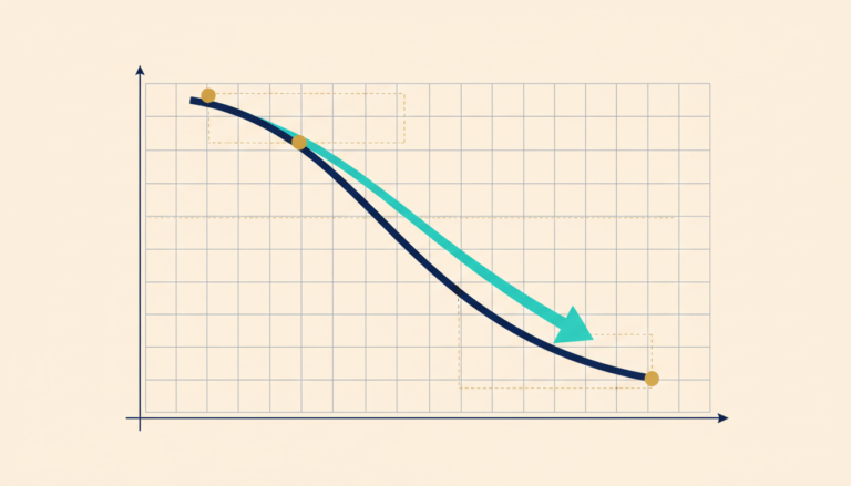
A straight line has a constant slope. A curve can become steeper or flatter as you move along it. The slope between two points is an average change over that interval; the local slope concerns the relationship very near a particular point.

Suppose total cost rises slowly at first, then more rapidly as a workshop approaches capacity and requires overtime. One average cost response across the whole range can hide the increasingly expensive additional output near the limit. The curve helps communicate that changing marginal relationship.

Do not infer the reason from curvature alone. Different mechanisms can produce similar shapes. A model should explain why the slope changes, while a data graph needs evidence supporting the proposed interpretation. Later mathematics introduces derivatives for local slopes, but the economic intuition can be understood before formal calculus is required.

8. Moving along a line differs from changing the line

In the cost model, completing more jobs while setup cost and unit cost remain fixed moves the outcome along the same line. Increasing setup cost from $30 to $50 shifts the line upward by $20 at every quantity. Changing unit cost from $4 to $6 changes the slope.

These changes have different meanings. A parallel shift does not imply a changed per-job cost in this particular model. A steeper line does. The graph can make the distinction clear when labels and scenarios are provided. This distinction is especially useful when learning how to read economic graphs that compare different assumptions or market conditions.

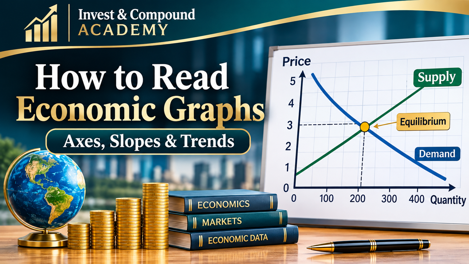
Demand and supply use a related distinction. An own-price change under fixed demand conditions corresponds to movement along the demand relationship. A change in another determinant can shift that relationship. The ceteris paribus topic develops the logic. Here, the visual skill is to ask which parameter or condition changed rather than describe every new point as a shift.

9. An intersection is a condition, not a universal solution

Two lines intersect where their coordinates satisfy both displayed relationships. In a market model, a supply-demand intersection can represent a quantity and price where planned buying and selling align under the model’s assumptions. In a cost-revenue graph, an intersection can represent break-even.

The intersection does not automatically establish fairness, stability or a desirable policy. Those conclusions require additional criteria and mechanisms. A diagram can show an equilibrium under restrictive assumptions without proving that an actual market reaches it quickly or that everyone benefits.

When reading an intersection, identify what each line represents and why satisfying both matters. Then examine feasibility and the domain. An algebraic intersection outside meaningful quantities is not a practical solution simply because the lines cross on a large enough canvas. Economic interpretation comes before attaching a label such as optimum.

10. Time-series graphs describe evolution, not automatic causation

A time series places observations in chronological order. It can reveal trends, cycles, abrupt changes and recurring patterns. It does not establish that an event marked on the timeline caused the subsequent movement.

Suppose sales rise after a service redesign. Seasonality, local demand or another business change may contribute. A vertical policy marker provides timing information, not a counterfactual. The correlation-and-causation topic explains what additional design is needed for attribution.

Check observation frequency and aggregation. Monthly, quarterly and annual averages can show different levels of volatility. A smooth annual line may conceal sharp movements within the year. That is not necessarily misleading, but the choice should match the question. A graph used to discuss short-run disruption needs enough temporal detail to represent the event being analyzed.

11. A scatterplot is not a timeline

A scatterplot shows pairs of observations, often for different people, businesses or locations. Points next to one another horizontally need not occur consecutively in time. Connecting them as if they form a path can suggest an order that does not exist.

Imagine plotting firms’ training hours against their average wages. The pattern may reflect differences in industry, worker experience, technology or firm size. An upward association does not isolate a training effect. The observational unit and sample definition are essential.

Inspect clusters and unusual observations. A relationship across all firms may differ within industries. One large or extreme observation can influence a fitted line. A responsible interpretation describes the visible association, then asks which comparisons and controls are justified. The picture can guide investigation without answering every causal question.

12. Zero is important in some charts and optional in others

A bar’s length usually represents magnitude, so truncating its baseline can distort the visual comparison. A line chart may use a narrower scale to reveal small changes, provided the axis is clear and the interpretation does not exaggerate the economic significance.

Suppose a rate moves from 4.0% to 4.2%. A vertical range from 4.0% to 4.2% makes the line span the entire plot. That can help inspect a small change but does not make the change enormous. A range from zero to 20% tells a different visual story with the same numbers.

Neither scale determines the correct economic conclusion. Report the actual change and relevant context. OpenStax’s mathematics appendix discusses how presentation choices such as axis ranges and selected dates affect perception. The reader’s task is to separate visual emphasis from numerical magnitude and substantive importance. Anyone learning how to read economic graphs should compare the displayed values, not rely on the apparent steepness of a line.

13. Percentage points differ from percentage changes

A rate rising from 5% to 6% increases by one percentage point and by 20% relative to its initial value. Both descriptions are correct, but they answer different numerical questions. A graph should indicate whether it plots a rate level or a rate of change.

Similarly, an index moving from 120 to 126 rises by six index points and 5%. Reading the vertical distance as a percentage without checking the starting value produces an error. The nominal-versus-real topic provides related examples of denominator changes.

When describing a chart, include the starting and ending levels if ambiguity is possible. That lets readers reconstruct the comparison. Avoid selecting only the more dramatic phrasing without explaining its basis. Precision about percentage points is especially important for interest rates, unemployment rates and shares of a population.

14. A growth rate differs from the level being grown

A graph of inflation displays the rate at which a price measure changes, not necessarily the price level. If inflation falls from 6% to 3%, prices can still be rising. A graph of output growth can fall while total output continues increasing at a slower pace.

To identify the meaning, read whether the axis shows dollars, an index, a percentage change or an annualized rate. A downward line in a growth-rate chart does not imply a declining level unless the rate becomes negative under the relevant convention.

This distinction prevents common headline errors. A slowing increase and an actual decrease have different implications. Where possible, compare the rate chart with the underlying level series and ensure their dates and transformations match. The two views can be complementary rather than contradictory.

15. Indexed lines compare relative movement

Suppose two businesses begin with revenues of $100,000 and $1 million. Setting both to an index of 100 in the first period allows comparison of subsequent percentage changes, but it hides the tenfold difference in initial size.

If both index lines rise to 110, both grew by 10%. Their dollar increases are $10,000 and $100,000. The indexed graph does not show equal absolute gains. It shows equal relative movement from the selected base.

Indexing is useful for comparing growth paths across differently scaled series. The base date still matters, especially if it is unusually high or low. A responsible presentation states the normalization and avoids using the lines to imply equality of levels. Readers should ask what information was intentionally removed to make the comparison possible.

16. Logarithmic scales emphasize proportional changes

On a logarithmic vertical scale, equal vertical distances correspond to equal proportional changes rather than equal arithmetic differences. A movement from 10 to 20 can occupy the same distance as 100 to 200 because both double. This can make long-run growth patterns easier to compare.

A log scale must be labeled. It is not appropriate for every purpose, and ordinary logarithms do not accept zero or negative values. Transformations used to accommodate such values require explanation rather than silently changing the meaning.

For a beginner, the main habit is to inspect tick spacing and labels. If the values rise by multiplicative steps, the visual slope has a different interpretation from an ordinary linear-axis graph. A curve on one scale may look straight on another. The underlying observations have not changed; the representation emphasizes a different comparison.

17. Dual axes require particular caution

A graph can place one series on a left axis and another on a right axis. The two scales may be chosen independently, allowing visually similar movement even when the numerical relationship is weak or difficult to interpret. The line crossing has no inherent meaning when the units differ.

Such charts can be useful if clearly designed for a specific purpose, but they require careful reading. Check each axis, the transformations and the reason the series appear together. A visual overlap does not establish equal levels, a stable relationship or causality.

Often separate aligned panels or a clearly normalized comparison are easier to understand. The appropriate choice depends on the question. The standard is whether the presentation helps readers evaluate the evidence rather than encouraging them to infer a relationship from arbitrary scaling.

18. Smoothing trades detail for readability

A moving average can reduce short-run noise and reveal a broader pattern. It also conceals some variation and can lag turning points depending on how it is calculated. A smoothed line should be labeled with its window and method.

Suppose daily deliveries are highly variable. A seven-day average can help compare underlying activity while reducing weekday patterns. It may nevertheless hide an important one-day outage relevant to reliability. A graph designed to discuss service continuity should not rely solely on the smooth average.

The choice is not between raw data being honest and smoothing being deceptive. Both can be appropriate. Explain why the transformation serves the question and retain enough information for readers to understand what was removed. If a conclusion depends on one specific smoothing choice, investigate its robustness.

19. Date selection changes the story

A series can rise over a decade, fall over the last year and fluctuate during the last month. Each statement can be true. A chart’s starting and ending dates determine which part of the story is visible.

Choose a window that matches the question and provide context when endpoints are unusual. Starting at a crisis low can make recovery appear exceptionally strong; starting at a temporary peak can make a normal correction look like persistent decline. Neither choice is automatically invalid, but the interpretation must acknowledge the baseline.

For comparison charts, align periods consistently. Do not compare one series from its trough with another from its peak unless the purpose explicitly requires it. A professional chart makes the comparison reproducible and gives readers enough context to evaluate whether the window supports the accompanying claim.

20. Uncertainty deserves a visual explanation

A forecast line can look definite even when its future path is uncertain. Bands or alternative scenarios can communicate uncertainty, but their meaning must be defined. A scenario range is not automatically a probability interval, and a confidence interval is not a promise about every possible future outcome.

Read the notes explaining how the band was constructed and what sources of uncertainty it includes. Parameter uncertainty, future shocks and model misspecification are different issues. A narrow band can omit important risks if the model is incomplete.

For an illustrative chart, clearly label assumed scenarios rather than using the visual conventions of statistical confidence without justification. For empirical forecasts, provide the method and appropriate caveats. The objective is to help readers understand what the evidence supports, not merely add a shaded area that creates an appearance of rigor. This matters when you learn how to read economic graphs that include forecasts, scenarios or uncertainty bands.

21. Read source notes and revisions

A graph should identify where the data came from, when they were accessed and whether they were adjusted or transformed. Official data can be revised as more information becomes available. A later chart may differ from an earlier release without either having been fabricated.

Check population coverage, seasonal adjustment and definitions. Comparing an adjusted series with an unadjusted one can create misleading differences. A change in classification can produce a break that resembles an economic event unless the notes explain it.

The source note is part of the argument. If the data are unavailable or the transformation cannot be reproduced, confidence should be limited. A sound method for how to read economic graphs therefore includes checking the source, definitions and revision history. A polished design cannot compensate for missing definitions. Reliable economic communication makes the underlying evidence inspectable rather than treating the chart as a self-contained authority.

22. Practice interpreting the cost model

At Q equal to ten, C equals 30 plus four times ten, or $70. At Q equal to fifteen, cost is $90. The slope between the points is $20 divided by five jobs, or $4 per job. The intercept remains $30.

Increase the intercept to $50 while leaving the slope unchanged. At ten jobs, cost becomes $90, a $20 upward shift. Alternatively, keep the intercept at $30 and raise the slope to $6 per job. Cost at ten is also $90, but the line changes differently at other quantities.

At twenty jobs, the first altered model gives $130 and the second gives $150. The same cost at one quantity does not imply the same underlying relationship. This is why inspecting several points and the model’s parameters is more informative than reading one crossing or one highlighted value.

23. Practice evaluating a chart claim

A headline says that unemployment exploded because a line rises sharply from 4.0% to 4.2%. The increase is 0.2 percentage points, or 5% relative to the initial rate. Its economic significance depends on context, uncertainty and the population, not the line’s angle alone.

Another chart shows two indexed revenues reaching 120 and claims equal dollar success. The claim confuses relative growth with absolute levels. A third shows prices and sales rising together and claims the price increase caused demand to rise. That inference requires a causal design and attention to shifting conditions.

For each case, identify the specific error and rewrite the conclusion accurately. This is more useful than calling a chart misleading without explanation. A reader should understand which inference fails and what additional information would be needed to support a stronger claim.

24. A repeatable graph-reading routine

Read the title, axes, units, source and period. Identify whether the figure shows data, a model or scenarios. Determine what one point represents and whether the scale is linear, indexed or logarithmic. Distinguish levels, growth rates and cumulative totals.

Then inspect slope, shifts, intersections and uncertainty according to the graph’s purpose. Check whether visual emphasis changes with axis ranges or endpoints. Ask whether the accompanying statement exceeds what the picture establishes, especially when it claims causality or welfare effects.

Finally, describe the result in a sentence containing the actual measure and comparison. If you cannot translate the picture into clear language, return to the labels and definitions. This repeatable routine makes how to read economic graphs a practical skill rather than a process of guessing from visual appearance. The goal is not distrust of every visualization. It is the ability to use graphs as transparent tools for reasoning rather than as substitutes for it.

25. Make the graph understandable without color or perfect vision

A useful economic graph should have readable labels, adequate contrast and a clear explanation of its main relationship. Distinguish series with direct labels or line styles rather than color alone. A reader using a small screen should not need to guess which axis or line is being discussed.

Provide a numerical table or concise text description when it helps readers inspect exact values. For an interactive model, explain which input changes the line and announce the resulting numerical output in accessible text. The graphic and the table should agree because they represent the same calculation. Clear labels, exact values and a short explanation make it easier to understand how to read economic graphs without confusing the illustration with observed evidence.

Accessibility also improves analytical quality. Writing a text description forces the author to state the measure, comparison and conclusion clearly. It also helps readers understand how to read economic graphs when color, screen size or visual detail is a limitation. If the graph’s message cannot be explained without relying on visual drama, the underlying claim may need clarification before publication.

References & Official Data Sources

• OpenStax, Principles of Microeconomics 3e, Appendix A — graphs, slopes and visual presentation.
• OpenStax, Principles of Economics 3e, §3.1 — demand, supply and market diagrams.

Examples and the interactive graph are hypothetical; no empirical dataset is used. Sources accessed October 22, 2026 UTC.