Invest & Compound Academy · Economic Thinking · Core Topic
Ceteris Paribus Explained: Meaning & Examples in Economics
Understand how economists isolate the effect of one changing factor by holding other relevant conditions constant—and why this analytical assumption matters when interpreting economic relationships.
Invest & Compound Academy · Core topic · Economic foundations and analytical methods
Isolate one relationshipExamine how a change in one variable relates to an outcome while other relevant factors are held constant.
Make assumptions explicitDefine which conditions remain fixed before drawing conclusions from a comparison or model.
Recognize real-world limitsUnderstand that many factors change together outside a simplified economic analysis.
The ceteris paribus meaning in economics is “other things equal”: holding other relevant conditions constant while examining a particular relationship. Economists use ceteris paribus to distinguish the effect of one change from changes occurring for other reasons. It is an analytical instruction, not a claim that the world stops changing or that inconvenient evidence can be ignored. In economics, this assumption helps demand and supply analysis separate the role of a product’s own price from other influences. [1]
Imagine a weekday lunch service increases its meal price and sells more meals afterward. That observation does not automatically show that customers prefer higher prices. More employees may have returned to nearby offices, a competitor may have closed or the menu may have improved. Several influences can move together, and their combined outcome can differ from the isolated effect of price.
This topic explains how to use the assumption responsibly. We will build an original hypothetical example around Linden Lunch, a small prepared-meal service. Its numbers are invented to make the reasoning transparent. They are not estimates of actual consumer behavior and should not be used to price a real business’s products.
Learning objectives
You will learn to identify the variable being changed, list the conditions being held fixed, distinguish a conditional effect from an observed change and interpret movements along a relationship versus shifts of that relationship. You will also learn why holding variables fixed in a spreadsheet is different from establishing a causal effect in data.
Suppose Linden Lunch wants to understand the effect of charging one additional dollar per meal. If the analysis simultaneously changes the menu, opening hours, customer population and price, the final sales change will combine all those influences. The owner may learn whether the complete package worked but not how price contributed.
Isolation helps answer a narrower question: how would customers respond to the price change under a specified set of conditions? That question is useful for reasoning even when an actual experiment cannot perfectly reproduce it. Once the isolated mechanisms are understood, the analyst can examine how they operate together.
Consider a different practical decision: whether reducing preparation time increases daily output. Holding staffing, equipment and product complexity fixed clarifies the productivity mechanism. If staffing also doubles, the total output increase cannot be attributed entirely to faster preparation. The principle is not restricted to prices; it applies whenever several influences could explain an outcome.
2. What “Other Things Equal” Really Holds Constant
No useful comparison holds every fact in the universe constant. Relevant conditions are those that could materially affect the relationship or its interpretation. For lunch purchases, they might include customers’ income, competing prices, product quality, nearby employment, weather and the time available to buy food.
The color of an unrelated building in another city is unlikely to matter for this question. Listing it adds complexity without improving the explanation. By contrast, a nearby employer adopting remote work could materially affect the number of potential customers. A careful analyst prioritizes plausible mechanisms rather than generating an endless list of conceivable influences.
Relevance depends on scope. Weather may be important for walk-in purchases but less important for scheduled deliveries. Income changes may matter differently for different customer groups. An assumption should therefore identify the particular market, population and period. “Other things equal” becomes more useful when the writer names the important conditions instead of leaving them entirely implicit.
3. Define the comparison before examining the result
A controlled comparison changes the variable under study while specifying the other relevant conditions that remain fixed.
A ceteris paribus comparison needs a baseline and an alternative. Suppose the baseline meal price is $12, the product is unchanged, and the service operates during the same weekday hours. The alternative price is $14 under otherwise specified comparable conditions. The comparison concerns the effect of the two-dollar price difference.
If the alternative also includes a larger portion, the product is different. The comparison may still be useful, but it no longer isolates the same-price-versus-new-price question for an unchanged meal. If the service adds delivery, convenience changes too. Those distinctions affect what the outcome can tell us.
Writing down the baseline prevents interpretation from shifting after results appear. If sales disappoint, the business should not retrospectively redefine success as customer awareness unless awareness was a stated objective and measured credibly. A transparent comparison identifies its outcome and important assumptions in advance, then reports what happened without quietly replacing the original question.
4. Build an explicitly hypothetical relationship
For teaching, assume weekly meal quantity Q follows this relationship: Q equals 160 minus 5 times P, plus 0.01 times the difference between Y and 3,000, plus 20 times Z. P is dollars per meal. Y is a hypothetical customer’s-group income measure expressed in monthly dollars. Z equals one when an additional nearby office is open and zero otherwise.
The relationship is deliberately simple. It assumes a constant price effect, a constant income effect and a fixed office-opening effect. It does not describe individual customers or capture every reason for buying lunch. We will use it only within a limited illustrative range, treating quantities as modeled meal volumes and bounding them below at zero.
At P equal to 12, Y equal to 3,000 and Z equal to zero, modeled quantity is 100 meals. This is the baseline. The equation is a controlled teaching environment: its inputs and mechanisms are known because we constructed them. Applying a similar equation to actual data would require justification, estimation and careful attention to causal interpretation.
5. Change price while holding other inputs fixed
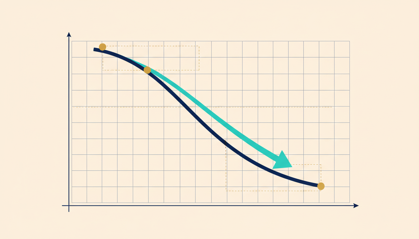
A change in the product’s own price produces movement along a demand curve when the other determinants of demand are held constant.
Increase price from $12 to $14 while leaving Y at 3,000 and Z at zero. Modeled quantity becomes 160 minus 70, or 90 meals. The isolated price effect is a reduction of 10 meals under the assumed relationship.
The calculation can also be written as negative five meals per dollar multiplied by a two-dollar increase. The units align: meals per dollar times dollars produces meals. That coefficient describes the relationship we assumed. It should not be presented as a discovery about real customers or a universal law governing all products.
This scenario illustrates the phrase other things equal. The result is conditional on the product, population, income input, office status and other modeled conditions remaining comparable. An actual observed sales change might differ because those conditions changed or because the model itself was unsuitable. The controlled calculation and the real-world observation are different kinds of evidence.
6. Change a nonprice condition while holding price fixed
Return price to $12. Increase the income input from $3,000 to $3,500, keeping office status unchanged. The model adds 0.01 times $500, or five meals, so quantity becomes 105. This represents a change in modeled demand at the same own price.
Now hold income at $3,000 but set office status to one. Quantity becomes 120 at the $12 price. The new office changes the market’s customer environment, so more meals are modeled at each price under the assumed equation. That is a different mechanism from customers responding to a change in the meal’s own price.
The distinction prepares readers for demand curves. A movement along a given demand relationship follows a change in own price under fixed relevant conditions. A shift represents a change in the relationship itself because another determinant changes. The visual treatment appears in the market chapters; here, the numerical comparison makes the logic explicit without requiring graph-reading skills.
7. Combine changes after understanding them separately
Suppose price rises from $12 to $14, income rises by $500 and the additional office opens. The model gives 160 minus 70 plus five plus 20, or 115 meals. Compared with the baseline of 100, price and observed quantity both rise.
The isolated price effect remains negative 10 meals. The income and office effects add 25, more than offsetting it. Under the constructed additive model, the combined change is positive 15. Observing higher sales alongside a higher price therefore does not identify a positive causal price response.
The decomposition works cleanly because we chose an additive relationship with constant coefficients. Real relationships can contain interactions and nonlinearities. The exercise establishes an important possibility, not an empirical diagnosis of every price-and-sales increase. To explain a real case, investigate what changed and whether the proposed mechanisms fit suitable evidence.
8. Some changes reinforce rather than offset one another
Suppose price increases while the relevant customer population shrinks. Under an ordinary downward-sloping demand relationship, the price increase reduces quantity demanded, and fewer potential customers can shift demand downward. The two mechanisms may reinforce one another, producing a larger sales decline than the isolated price effect.
That observation still does not reveal the size of each contribution. A business seeing a 20% sales decline cannot assign half to price and half to population without evidence. The mechanisms help organize the investigation; quantitative attribution requires appropriate information and a credible model.
This distinction prevents a common communication error: explaining direction and magnitude as though they were the same achievement. It may be reasonable to identify a plausible downward pressure while remaining uncertain about its strength. Professional analysis can say that several influences likely worked in the same direction, then identify the data needed to estimate their relative importance.
9. Interactions make the isolated effect conditional too
Our first equation assumes the same price response regardless of income or office status. Another model might allow price sensitivity to differ when customers have more alternatives or higher incomes. Then the isolated price effect depends on the starting conditions rather than one constant coefficient.
For example, imagine a hypothetical model in which a two-dollar increase reduces purchases by 12 meals when convenient alternatives are plentiful, but by six when alternatives are limited. Holding alternatives fixed remains useful, yet the conclusion must name which environment is being considered. There is no single effect independent of those conditions.
In mathematical terms, an interaction means that one variable changes the relationship between other variables. You do not need formal notation to understand the implication: ask not only what is held constant, but at what level. An average estimated response across several environments may conceal differences relevant to a particular decision.
10. Holding conditions fixed in a model is not random assignmentA model can hold conditions fixed by assumption; real-world evidence must still address the factors that change together.
A spreadsheet lets you change price while leaving other cells untouched. That produces a scenario under the spreadsheet’s assumptions. It does not establish that price was independently varied in the real world or that all omitted influences stayed unchanged.
An experiment attempts to create comparable conditions through design. Random assignment can help balance observed and unobserved characteristics on average, subject to implementation and other assumptions. An observational study must address why different people or periods faced different prices and whether those differences are related to outcomes for other reasons.
This is the boundary between an analytical comparison and empirical identification. Ceteris paribus states the effect we want to isolate. A research design explains why the available data can credibly isolate it. Confusing these steps lets a conditional story masquerade as a measured causal result. The next topic examines that problem in more depth.
11. A statistical control is not a magic guarantee
An analyst might include income and office status in a regression and call the price coefficient an effect holding those variables fixed. That interpretation depends on the model, measurement and causal structure. Relevant omitted factors, reverse causation or inappropriate controls can still distort the estimate.
Suppose Linden Lunch raises prices precisely on days when unusually high demand is expected. Price and sales then share a connection with expected demand. Including ordinary income information does not necessarily resolve that selection. The research design must address the reason prices vary, not merely add a long list of available variables.
Some controls can also remove part of the mechanism being studied. If a policy affects income and income affects purchasing, holding income fixed changes the question from a total policy effect to something narrower, if that narrower effect can be identified. Which variables to control requires causal reasoning rather than the assumption that more controls always improve a study.
12. Distinguish direct effects from full adjustments
Imagine a rise in an input cost increases a meal producer’s expenses. A narrow calculation may hold output and price fixed to isolate the immediate cost change. Over time, the business might alter portions, prices, suppliers or staffing. Customers and competitors may respond too.
The first calculation can be useful for understanding exposure. It is not the full equilibrium outcome after adjustment. Holding behavioral responses fixed answers a conditional question; allowing them to change answers another. Neither is automatically wrong, but the interpretation must match the model.
This distinction appears throughout economics. A household’s immediate payment change under a variable-rate contract differs from its eventual consumption response. A tax’s mechanical revenue calculation differs from revenue after behavior changes. To communicate responsibly, name whether the result is an initial arithmetic effect, an isolated behavioral response or a broader outcome that includes feedbacks.
13. Time horizons determine what can reasonably remain fixed
For tomorrow’s lunch service, kitchen capacity and the surrounding office population may be effectively fixed. Over several years, the business can expand or relocate, offices can change use and customers can adopt new routines. Assumptions suitable for a one-day comparison may fail for a long-run decision.
The phrase other things equal should therefore be connected to a time period. A short-run response often reflects limited adjustment options. A longer-run response can include investment, entry, substitution and institutional change. Those possibilities may amplify or reduce an initial effect depending on the mechanism.
Do not assume that the longer-run response must always be larger in every context. Specify the adjustments and the evidence supporting them. A model may predict a strong immediate reaction followed by adaptation, or a gradual response as contracts expire. The analytical task is to explain the path, not attach a universal rule to the words short run and long run.
14. The assumption should be open to challenge
A useful explanation states what evidence would call its assumptions into question. If customers change substantially, a previously stable demand relationship may no longer apply. If the product is redesigned, comparisons should acknowledge the quality change. If the business repeatedly misses predictions, the model should be reviewed.
Ceteris paribus becomes unhelpful when used to dismiss every observation that conflicts with a preferred theory. Saying something else must have changed is only a starting hypothesis. The proposed change should be identified, shown to be relevant and investigated where possible.
A responsible analyst distinguishes two questions: whether the conditional mechanism is plausible and whether that mechanism explains the observed event. A model can illustrate the first without establishing the second. Conversely, a surprising observation can reveal an omitted factor or a poor model. Treating evidence as a chance to improve the explanation is more productive than defending the original statement at any cost.
15. Apply the idea outside consumer demand
Consider training and employee output. Holding equipment, task difficulty and hours fixed helps isolate a proposed training effect. But employees selected for training may already be unusually motivated or skilled. A before-and-after increase could also reflect experience or a less demanding task mix. The analytical comparison must be connected to an empirical strategy.
Consider household commuting. A cheaper bus fare may reduce transport expenditure if route availability and travel patterns are fixed. If the household begins taking more trips, total expenditure may not fall by the mechanical amount. That does not make the fare calculation wrong; it means behavior changed the full outcome.
Consider interest expense. A fixed loan balance multiplied by a changed rate estimates an immediate exposure under specific contract assumptions. Repayment, refinancing and fees can alter the eventual amount. In each case, isolation clarifies a mechanism while the complete decision requires examining the adjustments that the initial comparison leaves aside.
16. Practice decomposing an observed change
Begin with Linden Lunch’s baseline of 100 meals. The price rises by one dollar, the income input rises by $200 and the office indicator stays at zero. Under our assumed equation, the price contribution is negative five meals and the income contribution is positive two. Modeled quantity becomes 97, a net decline of three.
Now suppose an actual business reports a decline of eight meals under superficially similar conditions. The difference does not reveal which factor is missing. Product quality, customer composition, competitor behavior, measurement error or an unsuitable relationship could contribute. The model gives a reference scenario, not a unique diagnosis.
A strong answer reports the calculation and its limits. It might say: under this teaching model, the two specified changes reduce quantity by three; explaining an actual eight-meal decline requires additional evidence. That wording preserves the value of the exercise without pretending the assumed coefficients were empirically established.
17. A checklist for reading “all else equal” claims
Identify the outcome and the variable being changed. Ask which important conditions are held fixed and whether their specified levels matter. Check the time horizon, population and domain. Determine whether the claim comes from a hypothetical model, an empirical estimate or an experiment.
Next, ask whether the proposed comparison is feasible and whether the analysis includes indirect adjustments. A statement about one product market should not automatically become a claim about national inflation or welfare. A short-run calculation should not silently become a long-run forecast. Units and boundaries matter as much as the phrase itself.
Finally, inspect how the author handles contrary evidence. Are alternative explanations named and investigated? Is uncertainty acknowledged? Can the assumptions be revised? An explanation that treats every outcome as confirmation is weak even if its terminology is correct. The purpose of the assumption is to make reasoning more precise and testable, not to protect a claim from scrutiny.
18. Practice explaining the idea in ordinary language
Imagine explaining Linden Lunch’s higher sales and higher price to a friend. A clear answer is: the price increase may have reduced purchases relative to what they otherwise would have been, while the new office brought enough additional customers to make total sales rise. The key comparison is with the alternative outcome under the same office conditions but the old price.
That sentence separates the observed change from the isolated effect. It does not need Latin terminology. It also avoids claiming that the exact contributions are known. To quantify them, we would need evidence about how customers respond and what changed during the period.
Using plain language is a useful test of understanding. If you cannot state which variable changes, what remains fixed and what comparison supports the conclusion, the phrase ceteris paribus may be hiding confusion. A professional explanation should make those elements easier to see, whether it uses an equation, a diagram or a short paragraph.
19. Write the limitation beside the result
When presenting a scenario, put the main assumptions near the output rather than burying them in a footnote. For example: the model predicts 90 meals at a $14 price, holding the income input at $3,000 and office status at zero. The coefficients are hypothetical, and the calculation excludes capacity and competitor responses.
This format helps readers understand what the result can support. It also makes the scenario reproducible: another person can enter the same inputs and check the arithmetic. If the analysis later changes an assumption, the reason should be recorded so the new result can be compared with the old one.
The broader habit is intellectual discipline. Isolate a mechanism when that helps, combine influences when the question requires it, and distinguish the model’s controlled environment from the data’s imperfect comparisons. Those habits prepare you for demand and supply, policy evaluation and the quantitative methods that appear later in the curriculum.
20. Interaction can make the order of decomposition matter
Our additive example permits a clean sum of separate changes. That convenience does not extend automatically to every relationship. Suppose a different teaching model sets quantity equal to an income-related spending amount divided by the meal price. When both income and price change, the quantity effect of the price change depends on which income level is used for the comparison.
Imagine the spending amount rises from $120 to $150 while price rises from $12 to $15. Quantity begins at 10 meals and ends at 10. If price changes first, quantity falls to eight and then rises by two when spending increases. If spending changes first, quantity rises to 12.5 and then falls by 2.5 when price increases. Both paths produce the same final total, but the separately assigned contributions differ.
This does not make the overall calculation inconsistent. It means that attributing a combined change to separate components can require an explicit convention when relationships interact. A professional decomposition should disclose the method rather than imply that one sequence-independent contribution exists for every variable. More advanced index-number and decomposition methods address related problems under defined objectives.
21. Comparable measurement is part of holding conditions fixed
Suppose Linden Lunch originally counts individual meals but later reports orders, some containing several meals. A change in the reported quantity would then combine behavioral changes with a changed unit of measurement. The comparison is not meaningful until the definitions are aligned.
Quality changes create a similar issue. A larger meal at a higher price is not the same product at a higher price. An analyst may attempt a quality adjustment, but the method needs justification. Simply asserting that all else is equal does not make changed products comparable.
Keep a record of the measurement rule, product definition and reporting period. If a week contains fewer operating days, compare like periods or explain the adjustment. If customer coverage changes, investigate the effect on the result. Good empirical practice begins with these ordinary details before statistical techniques are applied. Holding a concept fixed requires more than leaving a spreadsheet label unchanged.
22. Know when to widen the question
An isolated price response can inform a decision, but the owner eventually needs to compare complete feasible options. A $14 meal with better packaging and longer opening hours is a package of changes. The relevant decision may be whether to adopt that package, not whether price alone should rise.
Analyze the components where possible, then combine them using a coherent model and suitable evidence. Include the costs of implementation and the possibility that effects interact. The purpose of isolation is to improve understanding of the complete choice, not to prevent consideration of changes that necessarily occur together.
If the conditions cannot be held fixed operationally, state that limitation. A narrow theoretical effect may remain meaningful while being difficult to implement or estimate separately. Distinguishing conceptual clarity from practical feasibility helps readers understand both what the analysis teaches and what additional work an actual decision requires.
Interactive learning tool
The published Economic Thinking article introduces the broader framework of choices, incentives and constraints. This topic narrows the focus to one analytical instruction: compare two situations while holding other relevant conditions constant. The examples below distinguish a controlled model from real-world evidence.
Use the interactive tool below to change price, income and office status separately or together. Its outputs are hypothetical and show how simultaneous changes can be decomposed under the stated equation; they do not estimate real demand.
Separate simultaneous changes
Hypothetical Q = 160 − 5P + 0.01(Y − 3000) + 20Z, bounded below at zero. Coefficients are invented. Contributions add only where the zero bound does not bind.
Continue Learning with Invest & Compound Academy
Continue through the Economic Thinking chapter to see how economists isolate relationships, build explanations and assess evidence. The topics below connect this article to the wider foundations of economic analysis.
Ceteris Paribus Explained: What “Other Things Equal” Means in Economics
Correlation vs Causation in Economics: How to Evaluate an Economic Claim
Stocks and Flows in Economics: Measuring What Exists and What Changes
Nominal vs Real Values: Understanding Money and Purchasing Power
Efficiency vs Equity: Understanding Economic Outcomes and Fairness
The Fallacy of Composition: Why Individual Logic Can Fail for an Economy
Unintended Consequences in Economics: Looking Beyond the First Effect
How to Read Economic Graphs: Axes, Slopes and Changing Relationships
Explore the Earlier Market-Risk and Economic Pillars
These related Invest & Compound articles provide wider context on economic conditions, markets, financing and the evidence used to assess real-world claims.
Educational disclosure: This article provides general economics education and does not constitute personalized investment, tax or legal advice. The fictional transport scenarios, numerical assumptions and calculations are illustrative only and are not forecasts or reported research findings. Policy decisions require current evidence, jurisdiction-specific information and consideration of the people affected.
Linden Lunch, its equation and every numerical decomposition are original hypothetical instructional examples. The coefficients were chosen for teaching and are not measured elasticities, estimates or forecasts.
Explore the differences between microeconomics and macroeconomics through practical examples of business decisions, prices, wages, investment, inflation and economic growth. Learn how individual choices connect to economy-wide outcomes
The fallacy of composition explains why what works for one person, firm or market participant may produce a different result when many act together. Explore economic examples involving markets, congestion, saving, shared resources and financial markets.
Invest & Compound Academy · Economic Thinking · Core Topic What Is Economics? Understanding Choices, Resources and Society Explore how people, businesses and governments make choices, allocate limited resources and shape the economy. Scarcity Shapes Every Choice By Greg Roman · Educational research guide · Economic foundations and decision-making Choices under constraintsEconomics examines how people…
Learn correlation vs causation in economics through examples of confounding, selection, counterfactuals and research designs. Discover how to evaluate causal claims and evidence.
Explore the hidden costs of good intentions in economics. See how incentives, behavioral responses and policy decisions create unintended outcomes, shifted costs and second-round effects—and how to evaluate them.
Invest & Compound Academy · Economic Thinking Powerful Efficiency vs Equity Examples in Economics Explore how economics evaluates resource use and distribution—and…