S&P 500 Correction Frequency: How Often Do Declines Occur?

S&P 500 correction frequency is useful historical context, but it cannot tell you when the next decline will begin. Market corrections are among the most widely discussed—and frequently misunderstood—features of stock market investing. Whenever the S&P 500 declines sharply, investors begin asking whether the selloff is unusual. Financial commentators debate whether the market is experiencing a temporary interruption, the beginning of a prolonged downturn, or an attractive opportunity to purchase stocks at lower prices. One of the most useful ways to evaluate those questions is to examine the historical frequency of market corrections.

How often has the S&P 500 fallen 10% or more? Do meaningful declines happen every year? Are corrections becoming more common? How frequently do they develop into bear markets? And can the historical record help investors anticipate the next downturn? These questions sound straightforward, but the answers depend on how a correction is defined and measured. A conventional market correction begins when an index falls at least 10% from a recent peak. When researchers classify completed market declines, they often distinguish corrections that remain below 20% from bear markets that reach or exceed 20%.

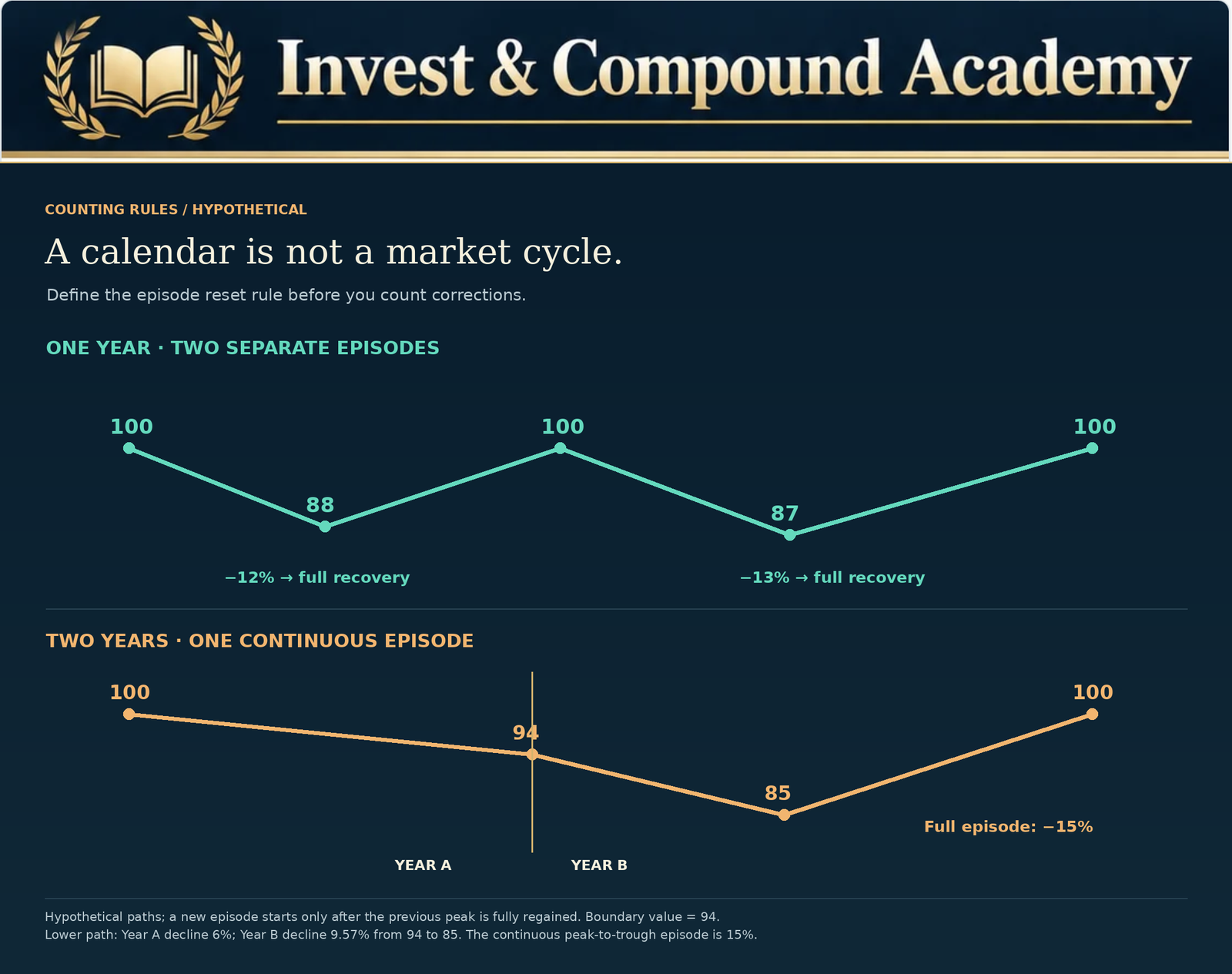
However, a historical study counting calendar years with a 10% intrayear decline answers a different question from one counting separate correction episodes. A year may contain several distinct declines. A single market downturn may extend across two calendar years. A correction may recover quickly, while another may evolve into a much deeper bear market. Consequently, claims that corrections happen a particular number of times per decade should be examined in the context of the data and methodology used. One widely cited finding comes from J.P. Morgan Asset Management’s historical analysis of the S&P 500.

Over the 46 calendar years from 1980 through 2025, the index experienced an average maximum intrayear decline of approximately 14.2%, even though 35 of those years finished with positive calendar-year price returns. These findings reveal an important characteristic of long-term equity investing: significant temporary losses have often occurred alongside positive annual market performance. They do not establish that the S&P 500 must experience a 14.2% decline every year, nor do they predict when the next 10% correction will begin.

Historical averages describe what occurred across a particular sample. They do not impose a predictable schedule on financial markets. This article examines how often S&P 500 corrections occur, explains the differences between drawdown statistics, discusses historical market examples, and shows how investors can interpret the evidence without confusing historical frequency with future certainty. Its central purpose is to replace vague claims about the normality of market volatility with a more precise understanding of what market statistics actually reveal.

What Is an S&P 500 Market Correction?

An S&P 500 correction refers to a decline of at least 10% from a relevant previous high in the index. Suppose the S&P 500 reaches 6,000. A subsequent decline to 5,700 represents a loss of 5%. If the index declines to 5,400, the cumulative loss reaches 10%. The market has entered correction territory under the conventional definition. If the decline continues to 4,800, the cumulative loss reaches 20%, the threshold commonly associated with a bear market. These percentages are measured relative to the relevant previous peak.

For a decline from 6,000 to 5,400:

This definition describes the magnitude of a price change. It does not determine how long the decline must last, what caused it, or whether the market will recover.

Corrections Are Defined by Price, Not the Economy

A market correction does not require a recession. Stock prices can decline because investors anticipate slower growth, higher interest rates, reduced profitability, or changes in risk preferences. Those expectations may later prove too pessimistic. As a result, a correction can occur while the economy continues expanding. Conversely, a decline that begins as a correction may deepen if business conditions deteriorate. The 10% threshold therefore describes an observed market movement rather than a definitive economic diagnosis.

The Importance of Consistent Reference Points

Historical market studies may use closing prices or intraday observations. The distinction matters when a decline approaches the 10% or 20% threshold. For example, an index might briefly fall 10.3% from its intraday high but finish the session only 9.8% below its previous closing high. An intraday study may identify a correction. A closing-price study may not. Neither observation is necessarily inaccurate. However, results from different conventions should not be combined as though they represent the same measurement.

For the broader mechanics, start with what a market correction is. The correction versus bear market guide explains the classification boundary. This article concentrates on how historical frequency is measured.

S&P 500 Correction Frequency: What Are We Counting?

Significant intrayear declines have been common over the S&P 500’s modern history. Research from major investment institutions shows that temporary drawdowns of 10% or more have appeared in many calendar years. However, the exact frequency depends on whether the analysis counts calendar years containing a qualifying decline or separately completed drawdown episodes. This is not a minor technical distinction. It can materially affect the answer.

Calendar-Year Frequency

An annual drawdown study usually calculates the largest peak-to-trough decline experienced during each calendar year. It then determines how many years contained a decline exceeding a specified threshold. This method is useful because it allows investors to compare annual market performance with the volatility experienced along the way. Suppose a hypothetical 20-year period includes twelve calendar years with a maximum intrayear decline of at least 10%. The observed frequency is:

The result indicates that 60% of the years in the sample experienced at least one qualifying intrayear decline. It does not indicate that twelve independent corrections occurred. Some years might have contained more than one qualifying episode.

Counting Separate Correction Episodes

A different method identifies successive market peaks and troughs. The researcher then counts separate declines reaching the correction threshold. This requires rules describing when one correction ends and another begins. For example, must the index regain its previous high before a new correction is counted? Does a partial rebound create a separate episode? How should researchers classify a decline that eventually becomes a bear market? Different decisions produce different historical totals.

Why Neither Method Is Universally Superior

Calendar-year analysis is particularly useful when evaluating the relationship between temporary losses and annual investment returns. Episode-based analysis is useful when examining the number, depth, and duration of distinct downturns. Both methods can support sound research. The problem arises when the resulting numbers are presented without explaining what they count.

For that exact count, use unrounded daily observations and a documented peak-and-recovery rule, or a source publishing the count under an explicit methodology. This article does not convert rounded chart labels into a precise 10% threshold count.

The Average Annual S&P 500 Drawdown

J.P. Morgan Asset Management’s Guide to the Markets provides a widely followed analysis of annual S&P 500 drawdowns. Its research for 1980 through 2025 reports an average maximum intrayear decline of approximately 14.2%. This figure can initially seem surprising. A market that has historically produced positive long-term returns has nevertheless experienced meaningful losses within individual years. There is no contradiction. Stock prices do not rise in a straight line.

What an Average Intrayear Drawdown Measures

The annual maximum drawdown describes the largest decline observed during that year under the specified methodology. For example, suppose an index begins the year at 100. It rises to 110, falls to 96, and eventually finishes at 118. The decline from the peak of 110 to 96 is:

Yet the calendar-year return is:

The market experienced a correction-sized decline from an intrayear high while finishing the year with a strong positive return. This is why annual performance figures can conceal substantial volatility.

What the 14.2% Average Does Not Mean

The average does not mean that the index declined exactly 14.2% each year. Some years experienced only modest losses. Others involved severe bear markets. The average combines many different observations. It is also not a statement that a 14.2% drawdown is equally likely in every future year. Financial conditions and market behavior change over time. Investors should interpret the figure as historical context rather than a forecasting target.

Source: J.P. Morgan Asset Management, Guide to the Markets – U.S., page 16, edition with data as of September 30, 2026. The completed-year summary covers 1980–2025; the separate 2026 YTD observation is excluded. The chart uses price returns, excludes dividends, and displays rounded annual values. The 14.2% mean and 35/46 count are the source’s published statistics, not estimates reconstructed from rounded labels.

For the difference between a return assumption and compounded wealth, see how compound interest works. Neither a historical average return nor an average drawdown describes a smooth year-by-year path.

Can Stocks Finish the Year Higher After a Correction?

Yes. One of the most important findings from historical S&P 500 research is that large temporary declines and positive annual performance are not mutually exclusive. J.P. Morgan’s 1980–2025 study found that the S&P 500 finished 35 of the 46 calendar years with positive price returns. That corresponds to approximately 76.1% of the observed years. At the same time, the average maximum intrayear decline was approximately 14.2%. The comparison shows that meaningful downside volatility can occur even in an overall favorable calendar year. However, it does not mean that every correction ended with positive annual returns.

Some years with severe declines finished deeply negative.

Why the Calendar-Year Starting Point Matters

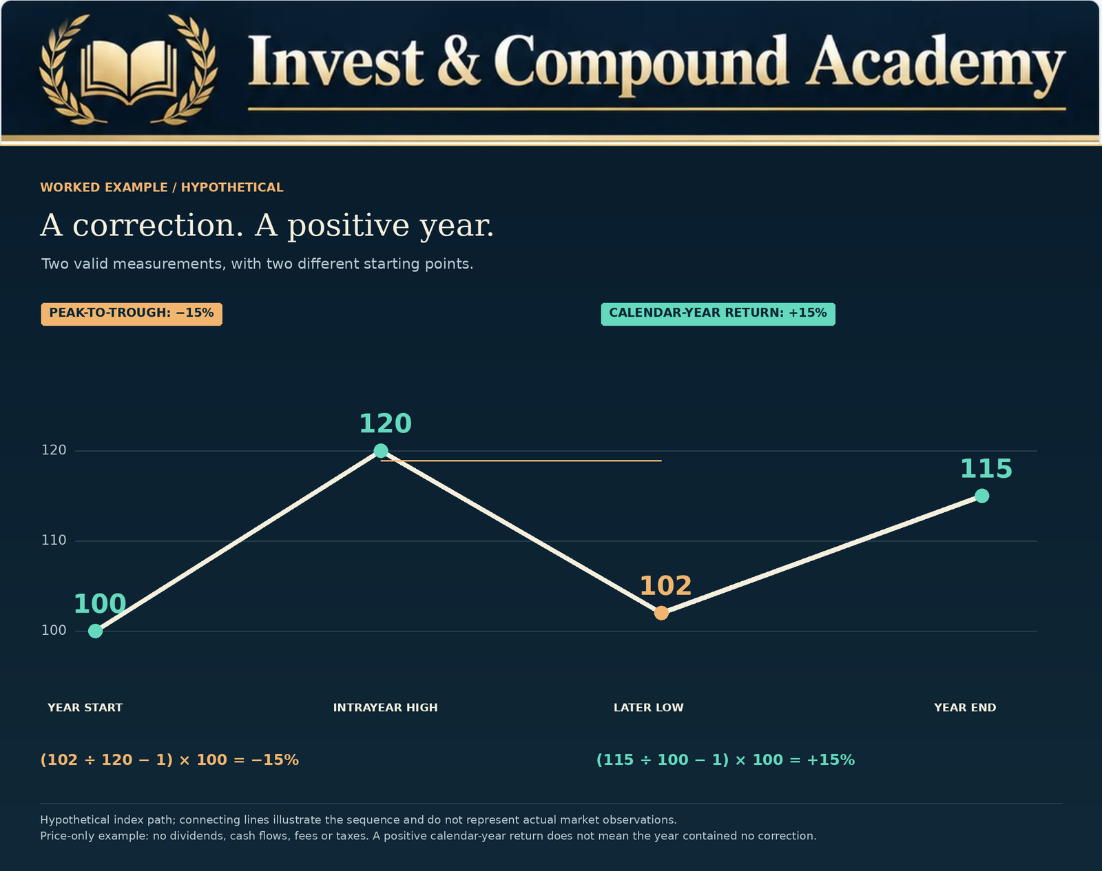
A calendar-year return is measured from the previous year-end value to the current year-end value. A drawdown is measured relative to a previous high. These reference points are different. A market can rise 20% early in the year, decline 15% from the new high, and still remain above its starting value. Consider an index beginning at 100. It rises to 120. A 15% decline reduces the index to 102. Even at the trough, the index remains 2% above its starting level. If it recovers to 115 before year-end, the annual return is 15%.

The peak-to-trough correction and the positive calendar return are both valid observations.

Why Investors Should Study Both Measures

Calendar-year returns are useful for evaluating investment performance over standardized periods. Drawdowns reveal the magnitude of losses investors may have needed to tolerate along the way. A strategy generating attractive returns but experiencing severe declines may be unsuitable for an investor requiring near-term capital. Conversely, an investor focusing exclusively on temporary drawdowns may underestimate the opportunity cost of repeatedly exiting the market. Both measurements contribute to a more complete understanding of investment risk.

How Often Do Corrections Become Bear Markets?

Some corrections remain within the 10%–less-than-20% range. Others develop into bear markets. A bear market is conventionally associated with a decline of at least 20% from a relevant previous peak. Every decline reaching 20% also qualifies as a decline of at least 10% under the same measurement convention. A sudden price gap can move directly beyond both thresholds without an observed trade at exactly 10% below the peak. However, not every correction continues to 20%.

Why the Conversion Rate Is Difficult to Define

Suppose a researcher identifies all dates on which the S&P 500 first falls 10% below a previous peak. The researcher then examines whether each episode subsequently reaches a 20% drawdown before fully recovering. This can produce a correction-to-bear-market conversion rate. However, the result depends on the rules for identifying episodes and determining when recovery occurs. If the researcher counts multiple repeated 10% declines within the same broader market cycle, the denominator changes. If each episode is required to begin from a new all-time high, the frequency may differ again. The study period also matters.

A sample including many severe historical bear markets may produce a different result from one focused on a relatively favorable period.

Why Investors Should Avoid Unsupported Probabilities

Claims that every correction has a fixed probability of becoming a bear market should be treated cautiously unless the underlying study is clearly identified. Historical conversion rates are conditional summaries of past observations. They are not universal probabilities. Economic conditions, valuations, monetary policy, and credit markets may influence the likelihood of deeper losses. A mechanically calculated historical percentage does not incorporate every relevant factor.

A Practical Interpretation

When the S&P 500 declines 10%, the market has demonstrated meaningful volatility. The decline may stabilize. It may deepen modestly. It may develop into a severe bear market. Investors should assess the financial consequences of several plausible outcomes rather than assume that historical averages identify the eventual low.

For deeper downturns, read the bear-market pillar. An annual maximum-drawdown average that includes bear-market years is not the average size of completed corrections restricted to losses below 20%.

Do Corrections Happen Every Year?

No. A market correction is a recurring phenomenon, but it does not occur according to a fixed annual schedule. Some calendar years do not contain a 10% decline under a given methodology. Other years experience multiple substantial episodes. Extended periods of relatively stable market advances can be followed by periods of unusually high volatility.

Why Corrections Cluster

Economic and financial risks are not evenly distributed over time. Inflation surprises, changing monetary policy, credit stress, and geopolitical uncertainty can contribute to repeated market movements. A year characterized by unstable interest-rate expectations may contain several significant declines. A different year may feature steady earnings growth and relatively low volatility. This creates clustering.

Why a Long Period Without a Correction Is Not a Countdown

Investors sometimes assume that the market becomes overdue for a correction after a prolonged advance. This resembles the gambler’s fallacy. The absence of a recent correction does not establish that a decline must occur within a specified period. Historical market events are not independent coin tosses governed by a fixed correction schedule. Nor are they governed by an automatic mechanism requiring a 10% decline after a certain number of trading sessions. The probability of a future correction depends on evolving financial conditions and uncertainty. A simple calendar count cannot capture those factors.

The Problem With “Corrections Happen Every Two Years”

Statements about one correction every two years may be shorthand for a particular historical average. However, averages do not imply regular spacing. Imagine a hypothetical ten-year period containing four corrections. Three occur within two consecutive years, followed by six years without one, and the fourth occurs near the end of the period. The average frequency is four episodes per decade. But describing them as occurring every two and a half years would conceal the actual pattern. Investors should distinguish long-run frequency from predictable timing.

Historical Periods of Elevated Market Volatility

Different economic eras have produced very different correction patterns. Examining selected periods reveals why correction frequency should be interpreted in context.

The Late 1980s

The 1987 stock market crash demonstrated how quickly prices can fall. Market structure, trading behavior, and liquidity pressures contributed to extraordinary volatility. The event shows why investors cannot assume that every decline will develop gradually. A severe downturn can occur before there is sufficient time to make orderly portfolio adjustments.

The 1990s

The 1990s included both significant market disturbances and a prolonged equity expansion. The 1990 downturn was associated with economic weakness, geopolitical uncertainty, and oil-price pressures. Later episodes included the Asian financial crisis and the 1998 emerging-market disruption. Yet these events did not prevent substantial equity gains across much of the decade. The historical record demonstrates that strong multiyear market performance can coexist with sharp temporary losses.

The Early 2000s

The collapse following the technology boom produced a much more severe environment. Broad U.S. equities entered an extended bear market. This period illustrates why a sample containing major financial crises can influence average drawdown statistics substantially. A 30% or 40% annual drawdown contributes much more to the average than a year with a 5% decline.

The Global Financial Crisis

The 2007–2009 financial crisis involved severe economic and financial-system stress. Credit deterioration, banking instability, and reduced confidence contributed to substantial equity losses. The experience demonstrates that a market decline can move far beyond correction territory. It also illustrates the difference between the duration of a decline and the time required to regain the previous peak.

The 2010–2011 Period

European sovereign debt concerns and U.S. fiscal uncertainty contributed to meaningful market volatility. The S&P 500 experienced deep corrections during this broader period. These episodes show how international financial developments can influence U.S. equity prices even when the original problems arise outside the domestic corporate sector.

The 2018 Corrections

The market experienced significant volatility in early and late 2018. Interest-rate expectations, inflation concerns, trade tensions, and uncertainty about economic growth influenced investor expectations. The late-year decline came very close to the conventional 20% bear-market threshold under closing-price measurement. This demonstrates that multiple substantial selloffs can occur within a single calendar year.

The Pandemic and Its Aftermath

The 2020 pandemic collapse was unusually rapid and developed into a bear market. The subsequent recovery was also unusually swift. Later, 2022 brought a different type of downturn, associated with inflation, rising interest rates, and valuation compression. These episodes illustrate why historical correction frequency alone cannot explain the financial environment. Different catalysts produce different market responses.

The historical market-corrections guide examines selected episodes and their measurement conventions. Separate the question of how often declines occur from how long corrections and their recoveries last; the bear-market duration guide covers deeper declines.

Are Corrections Becoming More Frequent?

This is a difficult question because it requires a consistent historical dataset and a clear definition of frequency. Changes in market structure, trading technology, financial regulation, investment products, and global connectivity may affect how information is incorporated into prices. However, the existence of algorithmic trading or exchange-traded funds does not establish that corrections must become more frequent. A sound statistical analysis would need to compare correction frequency across different periods using consistent price data and episode rules. It would also need to consider sample size and changes in market composition.

Why Recent Experience Can Mislead

Investors may perceive corrections as becoming more common after experiencing several turbulent years. This perception can reflect recency bias. Periods of volatility are particularly memorable. A calm market year may receive less attention. The number of prominent financial headlines is not a reliable measure of the statistical frequency of 10% drawdowns.

Why Historical Comparisons Are Difficult

Older market datasets may use reconstructed prices or different index methodologies. Changes in trading hours, index composition, market rules, and available historical data can complicate comparisons. Researchers should disclose the sample period and any limitations. Without this information, claims that the modern market is definitively more volatile may overstate the evidence.

What Can Be Said With Confidence

Corrections have repeatedly occurred under different market structures and economic conditions. They are not unique to modern electronic trading. The precise frequency of future corrections remains uncertain. Investors should avoid treating changes in trading technology as a substitute for measuring historical outcomes.

Why Corrections Are a Normal Part of Equity Risk

Equities represent ownership claims on businesses. Their market prices depend on expected earnings, future growth, discount rates, and risk preferences. These variables change continuously. A stock index therefore cannot reasonably be expected to rise at a constant rate.

Changing Earnings Expectations

Corporate profits fluctuate with economic demand, operating costs, competition, and industry conditions. Even when profits continue growing, they may fail to meet previously optimistic expectations. A broad reassessment of earnings forecasts can produce declining stock prices.

Interest-Rate Changes

Higher interest rates can increase borrowing costs and required returns. This may reduce the present value of expected future cash flows. However, higher rates can also reflect stronger economic conditions. The effect on equities depends on the underlying cause.

Changing Risk Preferences

Investors may become more or less willing to hold risky assets. When uncertainty increases, some investors demand greater compensation for equity risk. Valuation multiples can contract even before reported earnings deteriorate.

Unexpected Shocks

Geopolitical developments, public-health emergencies, financial failures, and policy changes can alter expectations rapidly. Markets may react before the full economic effects are known. These mechanisms help explain why volatility is a structural feature of equity investing rather than an unusual failure of the market.

For valuations, earnings, breadth, volatility and credit, see market correction warning signs. That guide distinguishes observable vulnerabilities from forecasts; a frequency statistic supplies no missing timing signal.

For a closer look at valuation changes, use P/E ratios explained. The guide to reading a stock’s financial numbers helps connect a lower share price with the earnings and balance-sheet information behind it.

S&P 500 Correction Frequency Versus Severity

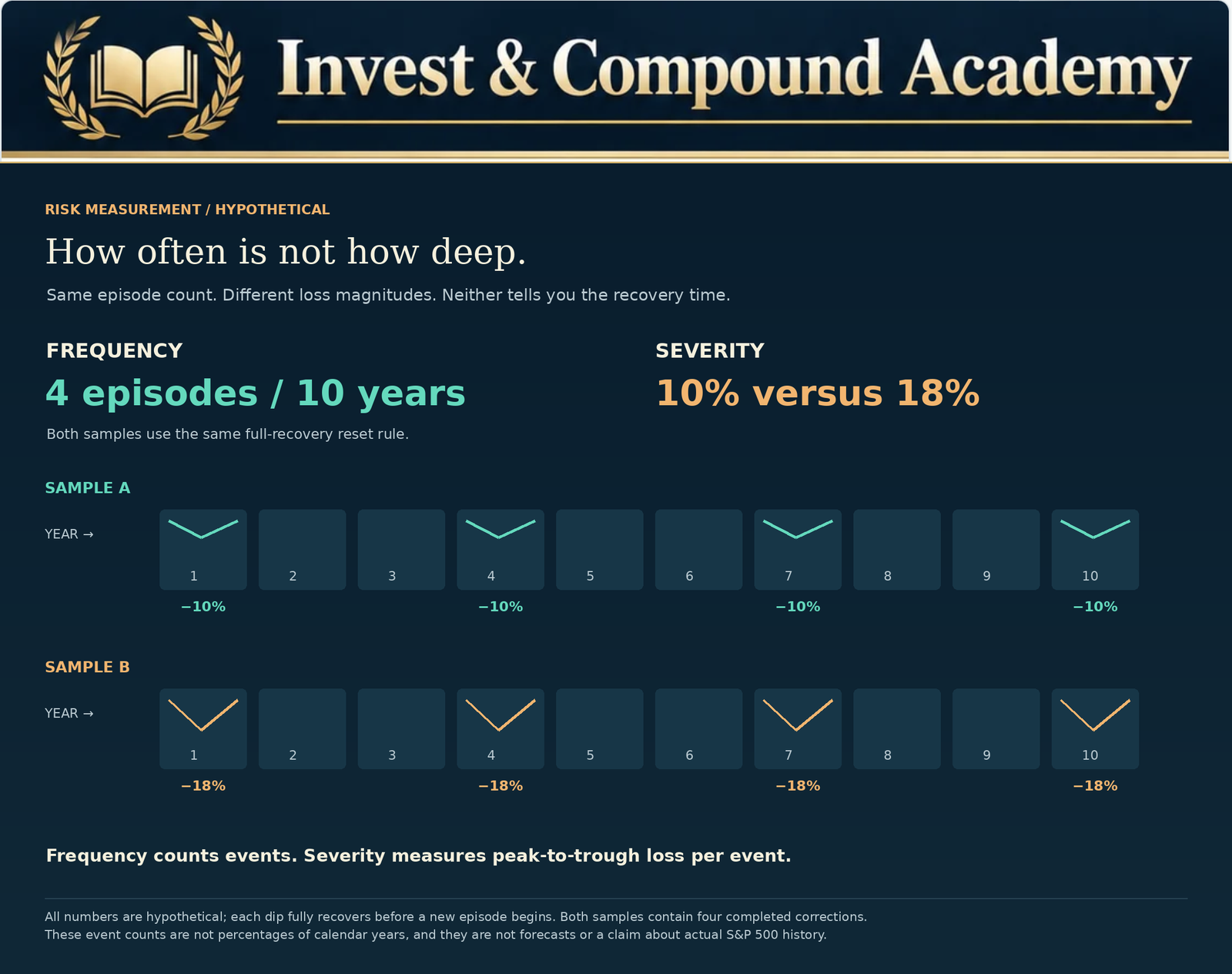
Frequency measures how often an event occurs. Severity measures the magnitude of the event. These concepts should not be confused. A market can experience numerous moderate corrections without suffering a prolonged catastrophic bear market. Another period may contain fewer distinct declines but include one exceptionally severe collapse.

A Hypothetical Comparison

Consider two separate ten-year periods. Period A contains six corrections with declines between 10% and 15%. Period B contains only three major declines, but one reaches 50%. Period A has more correction episodes. Period B contains a much more severe maximum drawdown. An investor evaluating risk based solely on frequency might conclude that Period A was more dangerous. That conclusion would ignore the greater loss severity experienced in Period B.

Why Both Measurements Matter

Frequent moderate declines can create psychological pressure and trading costs. Less frequent severe declines can threaten liquidity, leverage, retirement withdrawals, and financial objectives. A complete risk assessment should therefore consider both the number of declines and their magnitude.

Why the Average Drawdown Is Not the Expected Maximum Loss

The S&P 500’s historical average maximum intrayear decline of approximately 14.2% should not be treated as an estimate of the maximum possible loss. The word average is crucial. Some historical downturns have been much deeper. During the global financial crisis, major equity indexes experienced losses far beyond the ordinary correction range. The pandemic bear market also produced an exceptionally rapid decline exceeding 30%.

Tail Risk

Tail risk describes the possibility of unusually severe outcomes occurring in the extremes of a return distribution. Financial-market returns can display volatility clustering, abrupt jumps, and other characteristics that make simple probability models imperfect. A portfolio designed only around average market conditions may be poorly prepared for severe events.

Why Leverage Changes the Consequences

Consider an investor purchasing $100,000 in equities using $50,000 of personal capital and $50,000 of borrowed money. A 20% decline reduces the securities to $80,000. The loan remains $50,000, excluding interest. The investor’s equity falls to $30,000. A 20% decline in the underlying assets has produced a 40% loss of personal capital. Historical drawdown statistics must therefore be interpreted in relation to the investor’s actual portfolio structure.

Liquidity Matters

An unleveraged long-term investor may have greater flexibility to withstand a downturn. An investor facing margin calls or near-term cash obligations may be forced to sell. The same index decline can have different consequences depending on liquidity and financing.

Do More Corrections Mean Lower Long-Term Returns?

Not necessarily. The number of market corrections does not independently determine the long-term return of an equity index. Total investment performance depends on the full sequence of price changes and distributions. A period with several corrections can still produce substantial gains if the recoveries and subsequent advances are strong. Conversely, a period with relatively few corrections may produce disappointing returns if earnings growth and valuations remain weak.

Arithmetic Returns Versus Compounded Returns

Suppose an investment gains 20% in the first year and loses 20% in the second. Beginning with $10,000: After the first year, the value is $12,000. After the second year, it falls to $9,600. The arithmetic average return is zero. The compounded result is a 4% cumulative loss.

This illustrates why compounding differs from an arithmetic average. Without cash flows, changing the order of the same percentage returns does not change the ending value: 1.20 × 0.80 equals 0.80 × 1.20. The order becomes important when deposits or withdrawals occur.

Volatility Drag

When investment returns fluctuate, the compound growth rate can differ from the arithmetic average. Higher volatility can reduce compounded outcomes even when the arithmetic average appears favorable. However, volatility alone does not determine performance. Cash-flow timing, diversification, fees, and the level of investment returns all matter.

Long-Term Investors and Contributions

An investor making regular contributions may purchase more shares during periods of lower prices. Those purchases can participate in future gains if the underlying investment appreciates. However, regular contributions do not guarantee profits. The eventual outcome depends on the performance of the securities purchased.

The dividend yield versus total return guide explains why a price-only index chart is not a complete measure of an investor’s reinvested outcome.

To separate investment performance from money moving into or out of an account, read how to measure investment growth. Deposits can raise a balance during a loss, while withdrawals can lower it during a gain.

Can Corrections Be Used to Time Investments?

Historical frequency statistics are often used in attempts to predict when to buy stocks. An investor may reason that because corrections happen regularly, it is better to hold cash until the next one occurs. The difficulty is that corrections do not arrive on a predictable schedule. Markets may rise substantially while the investor waits. Even after a correction begins, the final bottom remains uncertain.

Waiting for a 10% Decline

Suppose an index trades at 100. An investor decides to wait for a 10% correction before buying. Instead, the index rises to 130. It then experiences a 10% correction from its new peak. The price falls to 117. The investor has waited for a correction but is now purchasing at a higher level than the original 100. This demonstrates the difference between buying below a recent high and buying below an earlier available price.

The Opportunity Cost of Waiting

Holding cash avoids immediate equity-market losses but also sacrifices potential equity gains while the money remains uninvested. The result depends on market performance and the return earned on cash. A waiting strategy can outperform if the market falls sufficiently before reinvestment. It can underperform if prices rise or recover quickly. Historical frequency alone cannot determine which outcome will occur.

Staged Investing

Some investors divide available capital into several purchases over time. This reduces immediate exposure to further declines but also delays participation in potential gains. The appropriate approach depends on risk capacity, investment horizon, and financial objectives.

Regular Contributions

Investors contributing from ongoing income may use fixed investment schedules. This reduces dependence on selecting one market entry date. However, the accumulated investment remains exposed to market risk.

For worked comparisons of immediate and staged purchases, see whether to buy stocks during a market correction. A discount from a later peak is not necessarily a discount from today’s price.

What Correction Frequency Means for ETF Investors

ETF investors frequently use broad-market funds for long-term wealth accumulation. An S&P 500 ETF offers diversified exposure to large U.S. companies, subject to the fund’s methodology. However, diversification within an equity index does not eliminate broad market risk.

Index Exposure

An S&P 500 ETF generally follows the index’s movements, allowing for fees, tracking differences, distributions, and other fund-specific factors. A 10% index correction can therefore produce a comparable decline in the market value of the ETF.

Sector and Growth ETFs

Technology-focused and growth-oriented ETFs may behave differently from the S&P 500. Their concentration and valuation exposure can lead to larger or smaller declines. The historical correction frequency of the S&P 500 should not automatically be applied to these funds.

Dividend ETFs

Dividend-paying investments can also experience substantial capital losses. Cash distributions do not create a guaranteed floor under share prices. Investors should evaluate total return and distribution sustainability.

Covered-Call ETFs

Covered-call strategies may generate option-premium income that partially offsets losses under certain conditions. However, the protection is limited and depends on strategy mechanics. Some approaches also sacrifice upside during strong recoveries. The frequency of S&P 500 corrections does not establish the return or distribution behavior of a covered-call fund.

Bond ETFs

Bond ETFs are exposed to interest-rate and credit risks. They may provide diversification in some equity downturns but can also suffer losses. The relationship depends on the economic environment and the bond portfolio’s characteristics.

The S&P 500 index guide explains the benchmark’s construction. Use the correct index and return series when comparing a fund with historical S&P 500 correction frequency.

For a concrete exposure comparison, see VOO versus QQQ. Our SCHD guide examines dividend-focused holdings, while SPYI explained examines an options-income strategy. Each has a different mandate; the S&P 500’s historical correction statistics are not interchangeable fund forecasts.

How Portfolio Allocation Changes Correction Exposure

An investor’s actual portfolio drawdown may differ from the S&P 500’s decline. Consider two hypothetical investors. Investor A holds a portfolio invested entirely in equities. Investor B holds 60% equities and 40% bonds. Suppose equities fall 20% while bonds remain unchanged. Investor A experiences a 20% portfolio decline. Investor B experiences a 12% decline. The calculation for Investor B is:

This example illustrates how allocation can influence portfolio losses. However, bonds do not always remain stable when equities fall. During periods of rising interest rates, stock and bond prices may decline together.

Diversification Is Not a Guarantee

Combining different assets can help distribute risk. But correlations are not constant. Investors should examine the conditions under which their investments may decline simultaneously.

Rebalancing

A correction may cause portfolio weights to drift away from target allocations. Rebalancing can restore the intended balance. Its primary purpose is maintaining desired risk exposure, not predicting the market’s next movement.

Matching Risk to Financial Objectives

A portfolio suitable for retirement savings several decades away may differ substantially from one intended to fund a near-term purchase. Correction frequency provides context, but asset allocation should ultimately reflect the investor’s financial circumstances.

Connect these scenarios with ETF portfolio construction and rebalancing with whole shares. For a broader portfolio review, read what to do during a market correction.

Several ETFs can still hold many of the same companies. The VOO and VTI overlap analysis shows how to look through the fund labels. Use the ETF portfolio review workbook to revisit concentration, allocation drift and maintenance decisions.

Why Retirees Experience Corrections Differently

Investors who regularly withdraw money from portfolios face additional challenges during declines. The order in which positive and negative returns occur can affect portfolio sustainability. This is known as sequence-of-returns risk.

A Withdrawal Example

Suppose a retiree begins with a $500,000 portfolio. A 20% decline reduces it to $400,000. The retiree then withdraws $25,000. The remaining portfolio is worth $375,000. Returning to the original $500,000 would require a gain of approximately 33.33%. Without the withdrawal, a 25% gain from $400,000 would have been sufficient.

This is the gain required to restore the original account balance after spending. The $25,000 withdrawal is not an investment loss: it funded living expenses. This single-withdrawal example illustrates the recovery hurdle, rather than simulating a recurring withdrawal schedule or a full sequence-of-returns analysis.

Why Frequency Matters Less Than Timing

A correction occurring decades before retirement may have different consequences from one occurring immediately after withdrawals begin. For retirees, the financial importance of a decline depends on when it occurs relative to spending requirements. The frequency of historical corrections is therefore only one component of retirement risk.

Liquidity and Spending Flexibility

Accessible reserves and flexible discretionary spending may help reduce forced selling. However, the appropriate approach depends on essential expenses, other income sources, taxes, and individual circumstances. No single retirement strategy eliminates sequence-of-returns risk.

The worked examples in compounding with withdrawals and return-sequence risk explore why spending changes the significance of return order. They address a different question from the number of corrections observed in a historical sample.

How to Interpret Correction Statistics Without Misusing Them

Historical correction data can be valuable, but investors should ask several questions before relying on a particular statistic.

What Index Is Being Measured?

The S&P 500 is not the same as the Nasdaq Composite, Russell 2000, or a global equity index. Each has different constituents, weights, and risk characteristics.

What Time Period Is Included?

A study beginning in 1950 may produce different results from one beginning in 1980. The observation period influences the frequency of major historical crises and favorable market environments.

Are Prices or Total Returns Used?

Price-index statistics exclude ordinary cash dividend reinvestment. Total-return calculations incorporate distributions. The distinction can affect returns and recovery timing.

Are Closing or Intraday Prices Used?

Intraday measurements may identify threshold crossings not visible in closing-price data.

Is the Study Counting Years or Episodes?

A year containing one or more 10% declines is not necessarily equivalent to one completed correction episode.

How Are Bear Markets Treated?

A study of all declines of at least 10% may include bear markets. A study restricted to corrections that remain below 20% may exclude them. Both methods can be valid for different research questions.

Are Numbers Rounded?

A decline of 9.96% may appear as 10% when rounded. A decline of 19.96% may appear as 20%. For classification near thresholds, the unrounded data matter.

Is the Statistic Descriptive or Predictive?

Historical observations describe previous market behavior. A forecast requires additional assumptions about future conditions. Confusing the two can produce unjustified confidence.

For a repeatable document-checking process, use how to research an ETF. Where an income fund is involved, the covered-call ETF financial-report guide helps separate distributions, per-share NAV and total return rather than treating cash payments as proof of recovery.

Building an S&P 500 Correction Frequency Dashboard

An educational dashboard can make historical statistics easier to understand. A useful research tool could allow readers to select a time period and threshold. For example, the reader might choose a 10%, 15%, or 20% maximum-drawdown threshold. The dashboard could then calculate the proportion of calendar years satisfying that criterion.

Useful Dashboard Outputs

The tool could show the number of calendar years analyzed, the number exceeding the selected drawdown threshold, the corresponding percentage, the average maximum intrayear drawdown, and the share of years finishing with positive returns. Each calculation should use the same underlying dataset.

Why Historical Data Must Be Transparent

Readers should know the index series, observation dates, price convention, and treatment of incomplete calendar years. A dashboard using rounded published chart figures can produce slightly different counts from one using unrounded daily observations. Those differences should be disclosed.

Avoid Invented Probability Claims

A historical frequency of 50% does not mean a correction has a 50% chance of occurring next year under all conditions. The historical sample is not a validated forecasting model. A professional tool should clearly distinguish observed frequency from predicted probability.

Why Interactive Calculators Improve Education

An interactive historical-frequency calculator can demonstrate how a statistic changes when the observation period or threshold changes. This helps readers understand why apparently contradictory research reports may both be reasonable. It also reduces the temptation to treat one historical average as a permanent market rule.

Common Misconceptions About S&P 500 Corrections

Corrections Happen Exactly Every Two Years

False. Historical averages do not establish a fixed interval between declines.

The S&P 500 Must Fall 10% Every Year

False. Some calendar years experience less than a 10% drawdown under a given methodology.

An Average 14% Drawdown Means a Maximum 14% Loss

False. Some historical episodes have involved much deeper declines.

A Positive Calendar Year Means No Correction Occurred

False. The market can experience a significant intrayear drawdown and still finish the year higher.

Every Correction Leads to a Bear Market

False. Some declines remain below 20% and subsequently recover.

Every Bear Market Begins With Months of Correction Activity

False. A sufficiently rapid crash can cross the 10% and 20% thresholds within days or even a single trading session.

Lower Prices Guarantee Better Investment Returns

False. Valuation, fundamentals, and future performance matter.

Correction Frequency Identifies the Best Time to Buy

False. Historical frequency does not establish a reliable market entry date.

Diversification Prevents All Market Declines

False. Broad equity-market risk remains even in diversified portfolios.

Every Individual Stock Eventually Recovers

False. Individual businesses can experience permanent impairment or bankruptcy.

Frequently Asked Questions

What Does S&P 500 Correction Frequency Tell Investors?

Historical research shows that declines of at least 10% have occurred regularly, but their exact frequency depends on the observation period and whether the study counts calendar years or separate episodes. They do not occur on a fixed schedule.

What Is the Average S&P 500 Intrayear Decline?

J.P. Morgan Asset Management reports an average maximum intrayear drawdown of approximately 14.2% for the 1980–2025 period.

How Often Does the S&P 500 Finish the Year Positive?

In J.P. Morgan’s 1980–2025 dataset, the S&P 500 finished 35 of 46 years with a positive calendar-year price return, approximately 76.1% of the observed years.

Does a 10% Correction Happen Every Year?

No. Some years experience smaller declines, while other years contain multiple substantial selloffs.

Can the Market Have Two Corrections in One Year?

Yes. Several distinct market declines can occur within a calendar year, depending on the methodology used to separate episodes.

Can a Correction Continue Into the Following Year?

Yes. Market peaks, troughs, and recoveries do not need to occur within one calendar year.

Do Corrections Always Become Bear Markets?

No. Some corrections recover before reaching the conventional 20% bear-market threshold.

What Is the Difference Between a Correction and a Bear Market?

A correction generally refers to a decline of at least 10% but less than 20%. A bear market occurs when the decline reaches at least 20%.

Are Corrections More Common Than Bear Markets?

Using the same peaks, recovery resets and observation window, the number of declines reaching at least 10% cannot be smaller than the number reaching at least 20%: the latter are a subset. Completed corrections restricted to 10%–less-than-20% form a separate category; their relative count must be measured, rather than inferred from the thresholds.

Are Corrections Becoming More Frequent?

A definitive answer requires a consistent historical dataset, methodology, and comparison across periods. Recent volatility alone is not sufficient evidence.

Can the S&P 500 Recover in the Same Year?

Yes. A market can experience a substantial intrayear decline and later finish with a positive calendar-year return.

Is a 10% Correction a Good Buying Opportunity?

It can create opportunities, but lower prices do not guarantee attractive value or positive future returns.

How Much Further Can Stocks Fall After a 10% Correction?

There is no fixed limit. A decline can stabilize or deepen into a bear market.

Should Investors Hold Cash Until the Next Correction?

That depends on financial circumstances, time horizon, and risk capacity. Waiting for a correction can involve significant opportunity costs if markets rise before the decline occurs.

Do ETF Investors Experience the Same Corrections as the S&P 500?

An S&P 500 ETF generally follows the underlying index, subject to expenses, distributions, and tracking differences. Other ETFs can experience substantially different drawdowns.

What Is the Most Important Statistic for Long-Term Investors?

No single statistic is sufficient. Historical returns, drawdown frequency, maximum losses, recovery periods, asset allocation, and liquidity needs all contribute to investment risk assessment.

Interpreting S&P 500 Correction Frequency Without Predicting Dates

S&P 500 market corrections are recurring features of long-term equity investing. Historical data show that meaningful temporary losses have occurred during many calendar years, including years that ultimately delivered positive returns. J.P. Morgan Asset Management’s analysis of 1980 through 2025 reports an average maximum intrayear decline of approximately 14.2%, alongside positive calendar-year price returns in 35 of the 46 years studied. The findings demonstrate that volatility and long-term market appreciation can coexist. However, they do not imply that a correction must occur every year or that a historical average can reliably predict the next downturn.

The frequency of calendar years containing a 10% drawdown differs from the number of separate completed correction episodes. The difference between closing prices and intraday observations can also change threshold classifications. Historical averages depend on the selected index, observation period, and methodology. These details are essential for interpreting market research accurately.

For investors, the practical lesson is that significant declines should be considered during portfolio construction rather than treated as extraordinary events requiring immediate predictions. An investor with a long horizon, appropriate diversification, sufficient liquidity, and manageable leverage may be better prepared to withstand volatility than someone whose financial plan depends on uninterrupted gains. However, no asset allocation or investment strategy guarantees positive results. Corrections can become deeper bear markets. Individual stocks can suffer permanent losses. Market recoveries can take longer than expected.

The purpose of historical analysis is not to eliminate these risks. It is to provide context for evaluating them. Rather than asking whether the market is overdue for a correction, investors may benefit more from asking whether their portfolio remains appropriate if one occurs. Rather than expecting the average drawdown to define future losses, they should recognize the possibility of more severe outcomes. And rather than attempting to forecast every turning point, they should establish financial processes that do not depend on successful short-term predictions.

Market corrections occur regularly, but they do not follow a reliable calendar. The more durable investment advantage is understanding their risks before they occur and maintaining a financial strategy capable of withstanding them.

Sources and Further Reading

Reference review: October 18, 2026. Historical summary: 1980–2025 completed calendar years. J.P. Morgan’s linked guide is updated periodically; the cited edition is dated September 30, 2026. Annual price returns exclude dividends. Rounded chart points do not support exact classification near thresholds. All other numerical examples and both calculators are hypothetical or user-supplied calculations.

1. J.P. Morgan Asset Management: Guide to the Markets – U.S., page 16, Annual Returns and Intra-Year Declines. Edition as of September 30, 2026; completed calendar years 1980–2025.
2. J.P. Morgan: Growth Fears Have Sparked Market Volatility. Earlier historical context; its observation window differs from the 1980–2025 summary.
3. S&P Dow Jones Indices: S&P 500 index overview and methodology.
4. SEC Investor.gov: Asset Allocation and Diversification.