S&P 500 Correction Statistics: Drawdowns and Recovery
Read historical losses with greater precision: distinguish event counts from time underwater, annual returns from drawdowns, and averages from extreme outcomes.
S&P 500 correction statistics help explain what investors have experienced, but their meaning depends on how the observations were measured. An average drawdown, a count of correction episodes and the proportion of days spent below a previous high describe different risks.
This guide examines those distinctions, the distribution of historical losses and the mathematics of recovery. To complement these S&P 500 correction statistics with a focused discussion of event frequency, read our S&P 500 correction frequency guide. Here, the emphasis is on interpreting the numbers without turning historical descriptions into forecasts.
The Benchmark Behind S&P 500 Correction Statistics
The S&P 500 measures large-cap U.S. equities using float-adjusted market-capitalization weights. Larger companies generally have more influence on its performance. It is not the entire U.S. stock market, a global equity portfolio or an unchanged collection of businesses.
Constituents and weights evolve. A diversified index can recover while an individual company suffers permanent losses or disappears. Index recovery statistics therefore cannot establish that a particular stock will regain its former price. Our guide to how the S&P 500 works explains its construction; the VOO and VTI overlap guide examines a practical benchmark distinction.
Live history and reconstructed history
The modern S&P 500 launched on March 4, 1957. Studies beginning in the 1920s use predecessor-index or reconstructed history for earlier observations. That history can be useful, but it is not a record of a live modern 500-stock index throughout the entire period. Check the provider’s series description before comparing studies.
Price returns and total returns
A price index measures changes in index levels without reinvesting ordinary cash dividends. A total-return index includes reinvested distributions under its methodology. Their recovery dates can differ. An ETF’s outcome also reflects expenses, tracking differences, taxes, currency exposure and investor cash flows. See dividend yield versus total return before comparing a price chart with an investor’s account.
The Mathematics Behind a Drawdown
A drawdown measures the percentage decline from a preceding reference peak. With a running-peak method, the reference is the highest observation recorded up to that date. When compiling S&P 500 correction statistics, the observation interval and starting date matter: daily closing data can miss intraday extremes, and a study beginning after an earlier peak may omit part of an existing decline.
Consider this hypothetical path: 100 → 108 → 115 → 110 → 103 → 98 → 105. The fall from 115 to 98 is −14.78%, even though the final level of 105 is 5% above the starting level. The annual return and the drawdown use different reference points.
Maximum drawdown is the deepest observed peak-to-trough decline in the chosen window. A multidecade maximum is not interchangeable with the average of individual annual maxima. Nor does a calendar-year calculation necessarily capture the full depth of an episode spanning December and January. Start with what a market correction means and the correction versus bear market comparison for the classification conventions.
What the Historical S&P 500 Correction Statistics Show
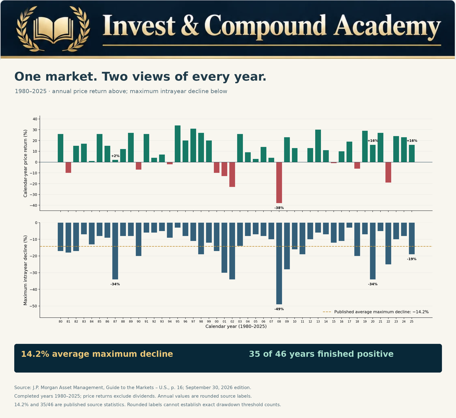
J.P. Morgan Asset Management’s published comparison reports a 14.2% average maximum intrayear decline and 35 positive calendar years out of 46 for 1980–2025. These are price-return observations, excluding dividends. The first describes the depth of annual declines; the second describes year-end outcomes.
The Academy chart below presents the annual observations chronologically. The completed-year sample excludes the separate 2026 year-to-date observation in the cited guide. Its annual labels are rounded; the two headline statistics are the provider’s published figures, rather than calculations inferred from those labels.
What the figures do not establish
Neither statistic counts separate correction episodes or establishes a probability for next year. An average loss is not a loss limit. Thirty-five positive years do not imply that the remaining eleven years each contained one correction, or that positive years avoided corrections.
The sample includes very different economic environments, and consecutive years are not identical independent experiments. Changing the start date, return series or peak convention can change a result. A longer sample includes more environments but may require reconstructed data; a shorter sample can be more contemporary while containing fewer observations.
S&P 500 Correction Statistics: Frequency, Severity and Duration
Frequency asks how often a defined event occurs. Severity asks how far prices fall. Duration asks how long the decline or recovery lasts. Useful market correction statistics consider all three rather than ranking investments using a single average.
In a hypothetical 25-year study, 13 qualifying calendar years give an observed frequency of 13 ÷ 25 = 52%. That does not establish that there were 13 separate correction episodes. One year may contain multiple episodes, while one episode may cross calendar boundaries.
Imagine one decade with five fully separated 10%–12% corrections and another with two drawdowns, one reaching 45%. The first has more events; the second has the deeper loss. Someone facing a near-term cash requirement may care especially about the largest loss and recovery duration, rather than which decade had the greater count.
How Thresholds Change S&P 500 Correction Statistics
Under common conventions, a 10% decline reaches correction territory and a 20% decline reaches bear-market territory. Completed corrections restricted to 10%–less-than-20% are a narrower category than all declines reaching at least 10%.
For the same observations and counting rules, raising a cumulative threshold cannot increase the number qualifying. A 25% drawdown belongs in an at-least-10% count and an at-least-20% count. In mutually exclusive severity bands, it belongs only in the 20%-or-more band. A price gap can cross thresholds without an observed trade at exactly either boundary.
| Maximum annual decline: hypothetical sample | Years |
|---|---|
| Less than 5% | 5 |
| 5% to less than 10% | 8 |
| 10% to less than 15% | 7 |
| 15% to less than 20% | 5 |
| 20% or more | 5 |
| Total | 30 |
Here, 17 of 30 years, or 56.67%, meet the cumulative 10% threshold. Five of 30, or 16.67%, meet the 20% threshold. These are invented observations for teaching the method, not historical S&P 500 counts.
Rounding can change a classification
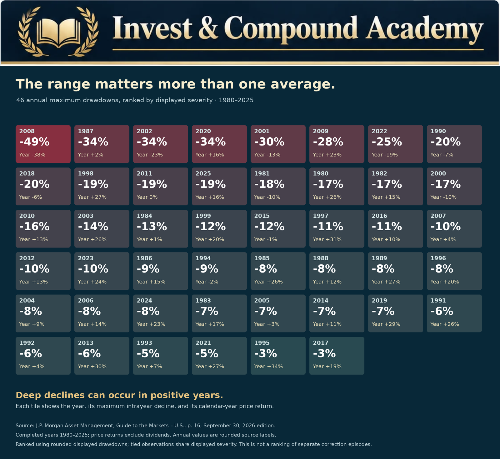
A 9.96% decline rounds to 10.0% without meeting an exact 10% threshold. A 19.96% decline similarly rounds to 20.0%. Use unrounded prices for threshold tests. The ranked historical illustration below uses rounded annual values to compare severity; it should not be used to assign borderline years to exact correction or bear-market categories.
Why Separate Episode Counts Differ
An episode-based study of S&P 500 correction statistics needs rules for selecting the starting peak, identifying the trough, resetting the count and handling an unfinished decline. A recent local high and an all-time high can produce different events. A 20% rebound from a low can mark a new phase under one convention without restoring the old peak under another.
For example, 100 → 87 → 96 → 82 contains an 18% decline from the original peak. Under a full-recovery reset rule, the rebound to 96 does not start a separate episode because the old high was never regained. A study of local selling waves could classify the same path differently.
An episode initially down 12% that later reaches 35% qualifies for a study of all declines reaching 10%. It would be excluded from a study limited to completed 10%–less-than-20% corrections. Report these choices before comparing counts. Our historical market corrections guide applies the same emphasis on explicit measurement conventions.
Bear Markets and the Severe End of the Distribution
Hartford Funds publishes a Ned Davis Research table covering 1929–2024, with 27 bear-market legs, an average decline of 35.24% and an average peak-to-trough duration of 289 calendar days. The last qualifying episode shown is in 2022. These figures use the provider’s cycle classification, rather than a universal full-recovery reset rule.
Its table splits parts of prolonged downturns into separate legs. Consequently, another study treating an entire collapse as one continuous episode can report fewer events and longer durations. The average measures the decline phase, not the full time needed to regain the old high.
The practical lesson is that losses can exceed an ordinary correction by a wide margin. It is not that a future bear market must match the historical average. Read our bear-market guide and bear-market duration research for fuller treatment of those questions.
Time Underwater Is Not an Event Count
Fidelity’s April 6, 2026 educational article states that, since 1927, the S&P 500 has spent more than one-third of the time at least 10% below a recent high. This is the provider’s historical time-share observation, not an independently reconstructed Academy episode count. The pre-1957 data caveat also applies.
Suppose an index is observed on 1,000 trading days and is at least 10% below its specified peak on 350 of them. Its observed time share is 35%. That does not mean 350 corrections occurred or that a new correction began on 35% of days. One prolonged episode can account for many observations.
This distinction in S&P 500 correction statistics explains why an investor can experience relatively few major downturns while spending substantial time below previous highs. That matters psychologically and can matter financially when withdrawals continue. It does not establish a 35% probability of a new correction tomorrow: a transition forecast requires a separate model and a defined current state.
S&P 500 Correction Statistics: Mean, Median and Extremes
Historical S&P 500 drawdowns should be examined as a distribution. The mean is the arithmetic average; the median is the middle ordered observation. For the hypothetical decline magnitudes 4%, 5%, 7%, 8%, 9%, 12%, 15%, 18% and 48%, the mean is 14% and the median is 9%. The unusually severe 48% observation lifts the mean substantially.
Percentiles add context, but their values depend on sample size and the interpolation convention. When losses are expressed as positive magnitudes, a high severity percentile describes unusually deep losses. Software working with negative signed returns can reverse the ordering, so disclose the sign convention as well.
Two datasets can share the same mean while having very different extremes. One may contain consistently moderate declines; another may combine mostly small losses with a few collapses. Neither an average nor a median is a worst-case boundary.
Annual return distribution answers another question
The stacked-year illustration below groups calendar-year price returns, not maximum drawdowns. Each block represents a year in a range based on the published rounded return. It is a useful companion to the S&P 500 correction statistics shown in the drawdown charts, but it cannot count corrections or reveal the path prices followed within a year. A displayed 0% may hide a small positive or negative unrounded return; use the source’s underlying precision for the 35-positive-year statistic.

Measuring Decline and Recovery Duration
| Measurement | What it describes |
|---|---|
| Peak to trough | Time from the reference high to the subsequent low |
| Trough to recovery | Time from that low until the reference peak is regained |
| Peak to recovery | The full underwater period, including decline and rebound |
A hypothetical 60-calendar-day decline followed by a 180-calendar-day recovery has a 240-calendar-day full underwater period. Calling it a 60-day recovery would omit most of the experience. Use consistent elapsed-day conventions so that the two components sum to the full interval.
Duration-based S&P 500 correction statistics require consistent units: trading sessions and calendar days are different. Price recovery and total-return recovery can occur on different dates. An unfinished episode has no observed full-recovery date and should not be silently removed from a study: doing so can bias recovery averages downward. Compare these definitions with how long market corrections last.
Recovery Mathematics After a Loss
After a decline, the same dollar gain must be earned on a smaller balance. Stock market recovery mathematics shows why the percentage required to recover is larger than the percentage lost.
| Decline | Remaining value of $100,000 | Gain needed to recover |
|---|---|---|
| 5% | $95,000 | 5.26% |
| 10% | $90,000 | 11.11% |
| 15% | $85,000 | 17.65% |
| 20% | $80,000 | 25.00% |
| 25% | $75,000 | 33.33% |
| 30% | $70,000 | 42.86% |
| 40% | $60,000 | 66.67% |
| 50% | $50,000 | 100.00% |
When translating S&P 500 correction statistics into recovery examples, these figures assume no cash flows, costs or separate distributions. They measure a recovery hurdle, not a recovery date. For constant positive annual growth r after a loss L, a smooth-compounding illustration gives years = ln[1 ÷ (1 − L)] ÷ ln(1 + r). Actual returns are uneven; the assumed rate is not a forecast. Our compounding guide explains the changing base behind the calculation.
A Positive Year Can Still Contain a Correction
Imagine a price index starting at 100, rising to 125, falling to 107.50 and ending at 118. Its peak-to-trough drawdown is 14%, while its calendar-year return is +18%. Someone buying at 125 finishes the year 5.6% below their purchase level, before costs and distributions.
The same index path therefore produces different investor outcomes depending on purchase dates and cash flows. Contributions during a decline buy at changing prices; withdrawals remove capital from the subsequent rebound. Dividends, fees, taxes and currency movements add further differences. Our guide to measuring investment growth separates account-balance changes from investment results.
Why Market Losses Cluster Across Economic Environments
Inflation, policy changes, earnings revisions and credit stress can persist across reporting periods. Falling collateral values can trigger margin calls, forced selling and liquidity pressure, reinforcing the initial decline. These mechanisms help explain why volatile observations can cluster instead of arriving on a regular calendar.
The early-2000s technology downturn, the global financial crisis, the pandemic and the 2022 decline occurred under different combinations of valuations, economic conditions and policy responses. Their recoveries are not interchangeable templates. Falling interest rates can support valuations, but can also signal weakening activity; the surrounding conditions matter.
An average within S&P 500 correction statistics provides broad context across different regimes while remaining limited as a conditional forecast. Subdividing the sample by regime introduces another problem: fewer observations in each group. Examine market correction warning signs for the distinction between observable vulnerability and a reliable timing signal. The P/E ratio guide and stock research guide explain the earnings and valuation assumptions behind prices.
Drawdowns, Average Returns and Compounding
An investment gaining 30% and then losing 20% has a 5% arithmetic average annual return. Yet $10,000 becomes $13,000 and then $10,400: 4% cumulative growth, or approximately 1.98% compound annual growth over two years.
The arithmetic average cannot be compounded as though it were a constant realized return. Reversing the same two returns without cash flows gives the same ending balance, because 1.30 × 0.80 equals 0.80 × 1.30. With deposits or withdrawals, the order can change the outcome.
This relationship is often discussed as volatility drag, but volatility is not the only determinant of results. Return levels, fees, taxes and cash flows also matter. Use S&P 500 correction statistics to evaluate drawdown depth and recovery duration alongside annualized performance and portfolio liquidity. A historically profitable portfolio can still be unsuitable for an obligation that falls due during a deep decline.
Applying S&P 500 Correction Statistics to ETF Portfolios
A broad U.S. equity ETF can provide index exposure with less single-company concentration, but it still carries market risk. A sector or growth-focused ETF may have a different loss distribution. Historical S&P 500 correction statistics are context for those funds, not a substitute for examining their holdings and strategy. Our VOO versus QQQ comparison illustrates that distinction.
Dividend payments do not guarantee capital preservation. The SCHD guide explains a dividend-focused approach, while SPYI explained examines an option-income strategy. Covered-call funds can retain substantial downside exposure and surrender some recovery upside. Compare total returns, rather than treating distribution rates as earned returns; our covered-call ETF financial reports guide shows where to investigate.
Bond funds introduce duration and credit risks of their own. They may diversify equity exposure under some conditions, but can also fall. Owning several overlapping equity ETFs does not necessarily provide meaningful asset-class diversification.
Connect the evidence with ETF portfolio construction, whole-share ETF rebalancing and the portfolio maintenance workbook. The ETF research guide helps evaluate whether a fund’s actual exposures match the risk being studied.
S&P 500 Correction Statistics and Retirement Risk
Suppose a retiree’s $600,000 portfolio falls 25% to $450,000. One $30,000 withdrawal leaves $420,000. A subsequent 25% gain produces $525,000. Even without the withdrawal, the same market returns would produce $562,500, because a 25% gain does not reverse a 25% loss.
The $37,500 ending account gap consists of $30,000 withdrawn and $7,500 of subsequent growth forgone. The withdrawal funded spending; it is not itself an investment loss. Adding that cash back without a return gives $555,000, compared with $562,500 for the untouched account.
This is a single-withdrawal illustration, not a full retirement simulation. With recurring withdrawals, the sequence of returns and the duration of depressed values can materially affect outcomes. Near-term reserves or flexible spending can change exposure to forced sales, but no structure guarantees success. See compounding with withdrawals and return sequence and what to do during a market correction for the practical planning questions.
A Research Checklist for S&P 500 Correction Statistics
| Research question | Measurement to check |
|---|---|
| How common are qualifying declines? | Calendar-year share or separately defined episode count |
| How severe are losses? | Distribution of drawdown magnitudes, not just the mean |
| How long does selling last? | Peak-to-trough duration with a stated day convention |
| How long is capital underwater? | Peak-to-recovery duration and unfinished episodes |
| Can positive years contain corrections? | Joint annual-return and drawdown observations |
| Are events evenly spaced? | Intervals between episodes under consistent reset rules |
| How sensitive are the findings? | Sample dates, median, percentiles and alternative conventions |
| Does the result apply to this portfolio? | Holdings, return series, currency, cash flows and costs |
For reproducible S&P 500 correction statistics, retain the data source, available date range, observation frequency, dividend convention, peak rule, recovery rule and treatment of incomplete episodes. Report pre-launch reconstruction and any missing observations. Classify exact thresholds using unrounded data, then round for display.
Educational Calculators: Counts and Portfolio Consequences
An application calculating historical S&P 500 correction statistics would need licensed or otherwise appropriately available price data and an explicit episode-identification method. The calculators here do not download historical data. The first evaluates counts supplied by you; the second translates a selected hypothetical loss into dollars and a recovery hurdle.
For the first tool, enter mutually exclusive severity-band counts from one consistently defined sample. Its defaults reproduce the invented 30-year table above. It reports cumulative threshold shares without double-counting within the exclusive total. A historical observed share is not a validated forecast probability.
For the portfolio tool, a hypothetical $125,000 balance falls to $112,500 after a 10% loss, $100,000 after a 20% loss, or $81,250 after a 35% loss. The corresponding required gains are 11.11%, 25% and 53.85%. The selected decline is a scenario, not an estimate of the next correction.
Common Misinterpretations to Avoid
- A 14.2% average drawdown is neither a 14.2% annual probability nor a maximum loss.
- Time spent underwater does not count new correction episodes.
- Calendar-year observations and peak-to-recovery episodes cannot be added together as though they were the same unit.
- A bear market belongs in cumulative at-least-10% counts, but not in an exclusive completed-correction band below 20%.
- Closing-price and intraday thresholds can produce different classifications.
- Rounded chart labels cannot resolve an exact boundary.
- A nominal price recovery does not necessarily restore purchasing power or an investor’s account after withdrawals.
- Past recoveries of a broad index do not establish that every security will recover or that a future recovery has a deadline.
Frequently Asked Questions
Average S&P 500 drawdown: what is being averaged?
The average S&P 500 drawdown within a year was approximately 14.2% in J.P. Morgan’s published 1980–2025 comparison. It averages annual maximum price declines, including severe years. It is not the average of completed corrections restricted to 10%–less-than-20%.
How many years in the sample finished positive?
The provider reports 35 of 46 calendar years with positive price returns. Use its underlying precision rather than attempting to reproduce the count from rounded labels, especially observations displayed as 0%.
Does the S&P 500 experience a correction every year?
No. Drawdowns recur, but a qualifying 10% decline does not occur on a fixed annual schedule. The chosen calendar-year and episode conventions affect reported frequencies.
Why do studies report different correction counts?
They can use different dates, index series, thresholds, reference peaks, recovery resets and observation intervals. Compare the methodology before interpreting a disagreement as an error.
Why examine both mean and median drawdowns?
An unusually deep loss can pull the mean above the median. Their difference helps describe the sample, while the full distribution and extreme observations reveal risks neither statistic captures alone.
Can a positive calendar year include a major correction?
Yes. A fall from a later peak can be large even when the year-end level remains above the starting level. Purchase timing and cash flows then create different individual outcomes.
What does stock market recovery mathematics tell us?
There is no fixed timetable. Distinguish the initial decline, the rebound from the low and the full underwater period. Confirm whether recovery uses prices, reinvested dividends or inflation-adjusted values.
Are corrections becoming more frequent?
A defensible answer requires comparable data and counting rules across periods, with attention to sample size. Recent volatility alone does not establish a persistent change.
Do correction statistics predict recessions?
They do not provide a reliable recession forecast by themselves. Market-price classifications and economic-cycle definitions measure different phenomena.
Can an ETF behave differently from the index?
Yes. Holdings, weights, leverage, option strategies, costs and currency exposure can change its loss and recovery profile. Verify what the fund actually owns and does.
Should investors wait in cash for the next correction?
That depends on obligations, investment horizon and risk capacity. Waiting can create opportunity costs, and a future correction may begin from prices above today’s. Our guide to buying stocks during a correction compares purchase timing, staged investing and valuation.
What is the main use of S&P 500 correction statistics?
They help explain the range and structure of historical risk. They do not identify the next downturn’s date, depth or recovery time. Use them to test assumptions about a portfolio, rather than to manufacture certainty.
Turning Historical Evidence Into Better Questions
Useful S&P 500 correction statistics begin with a defined question: how often, how deep, how long, or what happened to an investor’s money? Different measurements answer those questions, and none can replace the others.
Before acting on a market statistic, identify its sample, reference peak, return convention and counting rule. Then ask whether your own holdings, cash needs and time horizon resemble the exposure being measured. The value of the research is a more realistic understanding of risk—not a reliable calendar for the next correction.
Explore the Earlier Market-Risk Pillars
Use the full series to connect statistical interpretation with definitions, historical episodes, duration, market indicators and portfolio decisions.
Continue Learning in the Invest & Compound Academy
Explore the related questions without confusing event frequency, loss severity and recovery duration.
Market risk, indexes and portfolio strategy
Market Correction Pillar | Indexes and Markets | Portfolio Construction
Sources and Further Reading
Reference review: October 18, 2026. Historical windows differ by source and are identified beside the relevant statistics. The linked J.P. Morgan guide is updated periodically; the cited edition is dated September 30, 2026. Its separate 2026 YTD observation is excluded from the 1980–2025 illustrations. Annual chart values are rounded and price-only. All invented datasets, portfolio examples and calculator defaults are explicitly hypothetical.
- J.P. Morgan Asset Management: Guide to the Markets – U.S., page 16. September 30, 2026 edition; completed-year chart observations 1980–2025.
- Fidelity: What Is a Market Correction? April 6, 2026. Source of the attributed historical time-share statement.
- Hartford Funds / Ned Davis Research: Bear-market table, 1929–2024. Source dated March 2025; last listed qualifying bear episode in 2022.
- S&P Dow Jones Indices: S&P 500 index overview and methodology.
- S&P Global: March 9, 2021 historical note confirming the March 4, 1957 launch.
- SEC Investor.gov: Asset Allocation and Diversification.
This article provides general financial education and information, not personalized investment, financial, legal or tax advice or a recommendation to buy, sell or hold a security.
Historical correction statistics depend on sample dates, index construction, return series, observation intervals, thresholds and event-reset rules. Pre-launch observations can use predecessor or reconstructed history. Descriptive frequencies are not validated forecast probabilities, averages are not maximum-loss limits, and historical recovery does not establish a future deadline.
Investments can lose principal permanently. Diversification, rebalancing and regular contributions do not eliminate market risk. Past performance does not guarantee future results. Consider your circumstances and consult qualified professionals where appropriate.