Lump-Sum Investing vs DCA: Returns, Costs and Risks
Compare investing available cash immediately with a defined staged schedule, using matched price paths, historical research and two interactive calculators.
Lump-sum investing puts available investment capital into the chosen portfolio immediately. Staged investing, often called dollar-cost averaging or DCA, divides that same cash across predetermined purchase dates. The comparison is about when money enters the market—not how to invest savings that have not yet arrived. If prices rise while some cash waits, later purchases buy fewer shares. If prices fall, staged purchases can acquire more shares and reduce the initial loss. Neither path is known in advance, and a smaller loss is still a loss.
This guide compares the methods using the same starting capital, explains cash interest and trading costs, and examines historical research without treating it as a forecast. Four worked illustrations and two calculators make the assumptions visible. For the separate question of regular contributions and average acquisition cost, see dollar-cost averaging explained.
The Essential Difference Between the Strategies
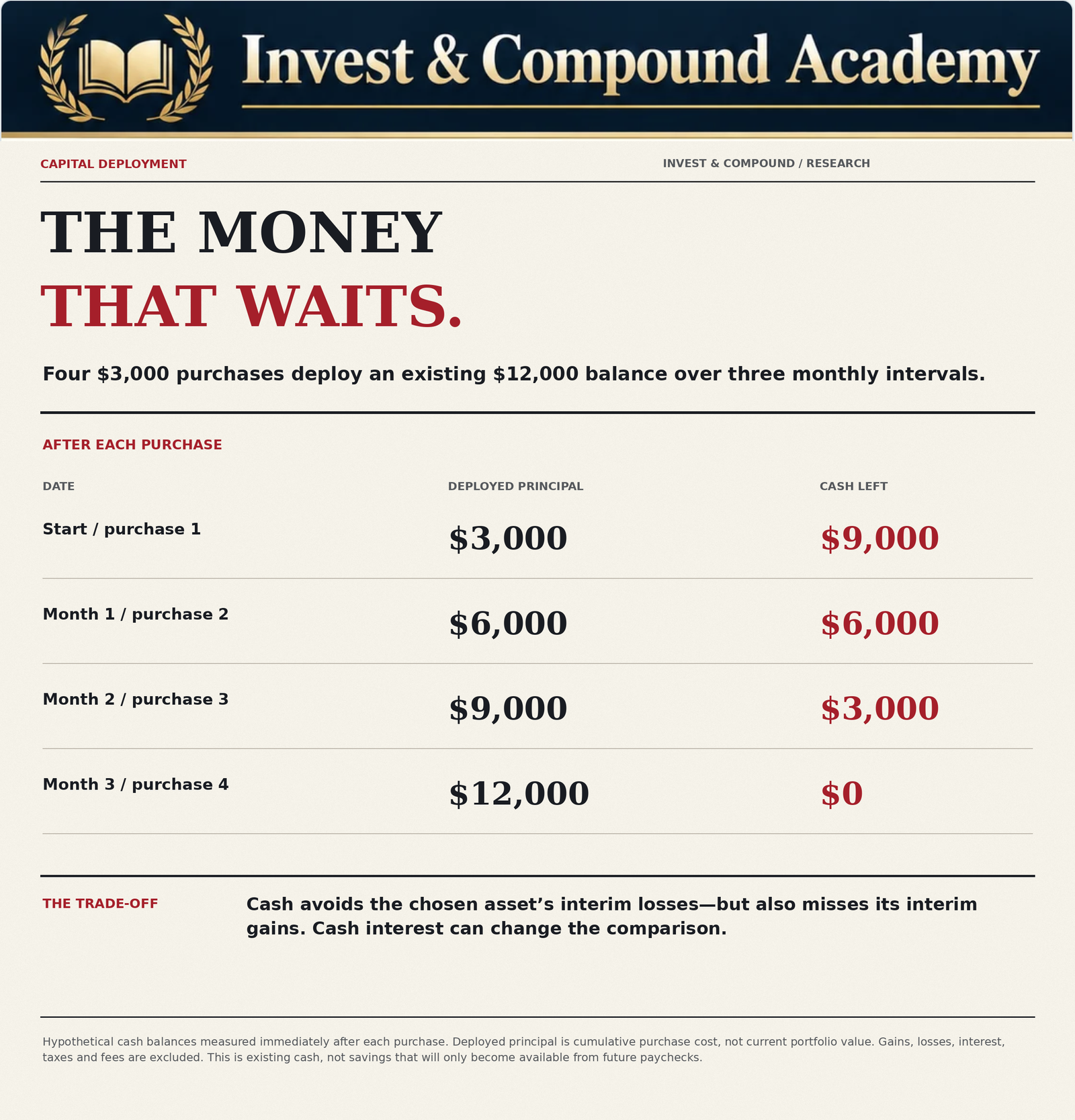
Lump-sum investing and staged investing differ primarily in when an investor accepts market exposure. Suppose an investor has $12,000 available and intends to invest it in a broad-market equity ETF. Under a lump-sum strategy, the entire amount is committed at the beginning. Under a four-purchase monthly dollar-cost averaging schedule, the investor invests $3,000 initially and then makes three additional monthly purchases of $3,000. The first purchase is made immediately; the fourth follows three monthly intervals later. At the end of the fourth purchase, both strategies have committed the full $12,000.
However, they may own different numbers of shares because the purchase prices changed.
Lump-Sum Investing
Lump-sum investing is the immediate deployment of available capital according to a selected investment allocation. It does not necessarily mean putting every dollar into one stock. An investor might divide $50,000 into a diversified portfolio of stock and bond ETFs on the same day. The defining feature is that the intended allocation is funded immediately.
Dollar-Cost Averaging an Existing Lump Sum
In this comparison, dollar-cost averaging means deliberately dividing capital already available into multiple investments made over time. The purchase schedule is determined in advance rather than being adjusted to predict the next market movement. For example, an investor might invest one-quarter of the available balance on each of four monthly purchase dates.
What Is Not Being Compared
Investing $500 from each paycheck is often described as dollar-cost averaging. However, that situation differs from holding back $12,000 already available. Someone who receives wages over time may not have the future contributions available for immediate investment. The choice between lump-sum and staged deployment applies most directly when a specified amount of capital can be invested today but the investor is considering postponing part of the purchase. That distinction prevents a common analytical mistake: treating regular saving from future income as though it always involves an avoidable delay.
The dollar-cost averaging guide develops regular contributions, average cost and whole-share purchases. Here, the starting cash is already available. Keep that distinction when interpreting a lump-sum investing comparison.
Why Immediate Investment Has Historically Had an Advantage
The expected-return argument for lump-sum investing is straightforward. If an asset has a positive expected return over the relevant horizon, an investor generally gains more expected exposure by owning it sooner. A staged investor temporarily allocates part of the intended investment to cash. That cash may earn interest, but its expected return may differ from the expected return of the selected portfolio. When the expected return on the investment exceeds the after-cost return on cash, holding back capital creates an expected opportunity cost.
Positive Expected Returns Are Not Guaranteed Returns
Equities have historically provided returns that compensate investors for bearing economic and market risks. But an expected return is not a promise. The next day, month or year can deliver substantial losses. The distinction between expected and realized outcomes is essential. An investor may make a decision with a higher expected return and still experience the worse actual result. That does not automatically mean the original decision was irrational. It means uncertainty was present.
Time in the Market
A lump-sum investment provides full exposure from the beginning. A staged investment increases exposure gradually. Suppose an investor spreads $12,000 across four equal monthly purchases. Immediately after the first purchase, only 25% of the eventual capital is invested. After the second purchase, 50% has been committed. After the third, 75%. Only after the fourth purchase is the portfolio fully invested. The investor’s average exposure during this period is therefore lower than under immediate deployment. If markets rise, that difference typically benefits the lump-sum investor.
If markets decline, it can benefit the staged investor.
Cash Drag
Cash drag refers to the effect of holding part of an investment portfolio in an asset with a lower return than the intended investment. It is not necessarily a mistake. Cash may provide valuable liquidity and risk reduction. However, when cash is held solely because an investor hopes for a better future entry price, the delay should be recognized as an active capital-allocation decision. The investor is temporarily choosing more cash and less exposure to the intended portfolio.
Our investment-growth measurement guide separates new money from gains. The compound-interest guide explains how a larger invested balance can affect later dollar outcomes without guaranteeing a positive return.
What the Vanguard Research Actually Found
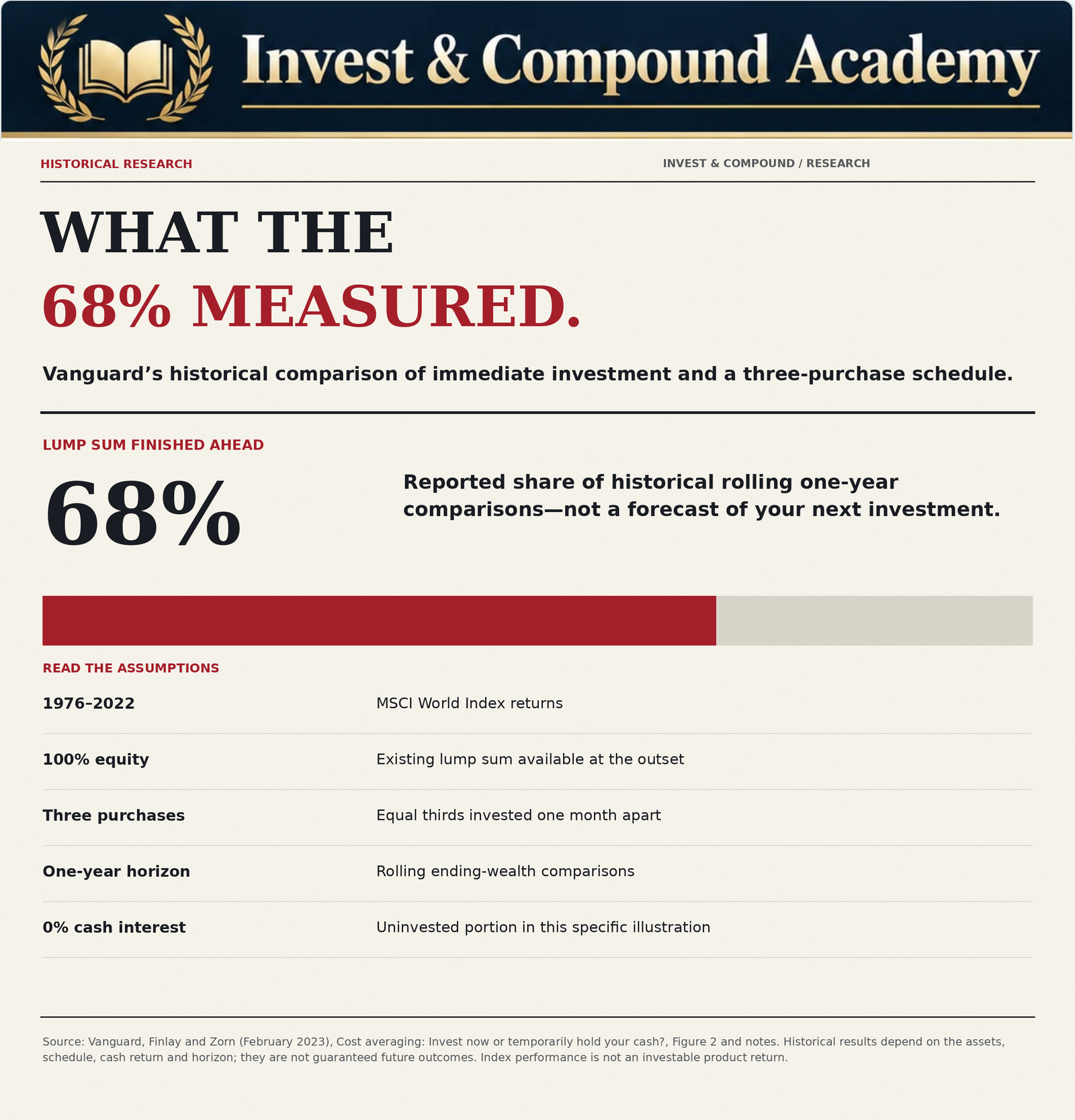
Vanguard’s February 2023 paper by Megan Finlay and Josef Zorn compares deploying available capital immediately with staged investment. Its Figure 2 global-equity illustration reports that lump sum finished ahead in 68% of rolling one-year comparisons using MSCI World returns for 1976–2022. That illustration assumes 100% equity, three equal purchases one month apart, and no interest on the uninvested portion. It does not compare investing an available lump sum with investing future paychecks. Nor does 68% measure the size of the return advantage or the probability of a profitable investment.
Changing the allocation, deployment dates, cash return or outcome horizon changes the question being tested. The result supports an expected-return argument for earlier exposure; it does not promise the better outcome in an individual case. The research also discusses loss aversion. A defined staged schedule may help an investor implement an otherwise suitable plan, while temporarily reducing market exposure. That behavioral benefit must be weighed against delayed participation in potential gains.
Scenario Analysis: A Market That Rises
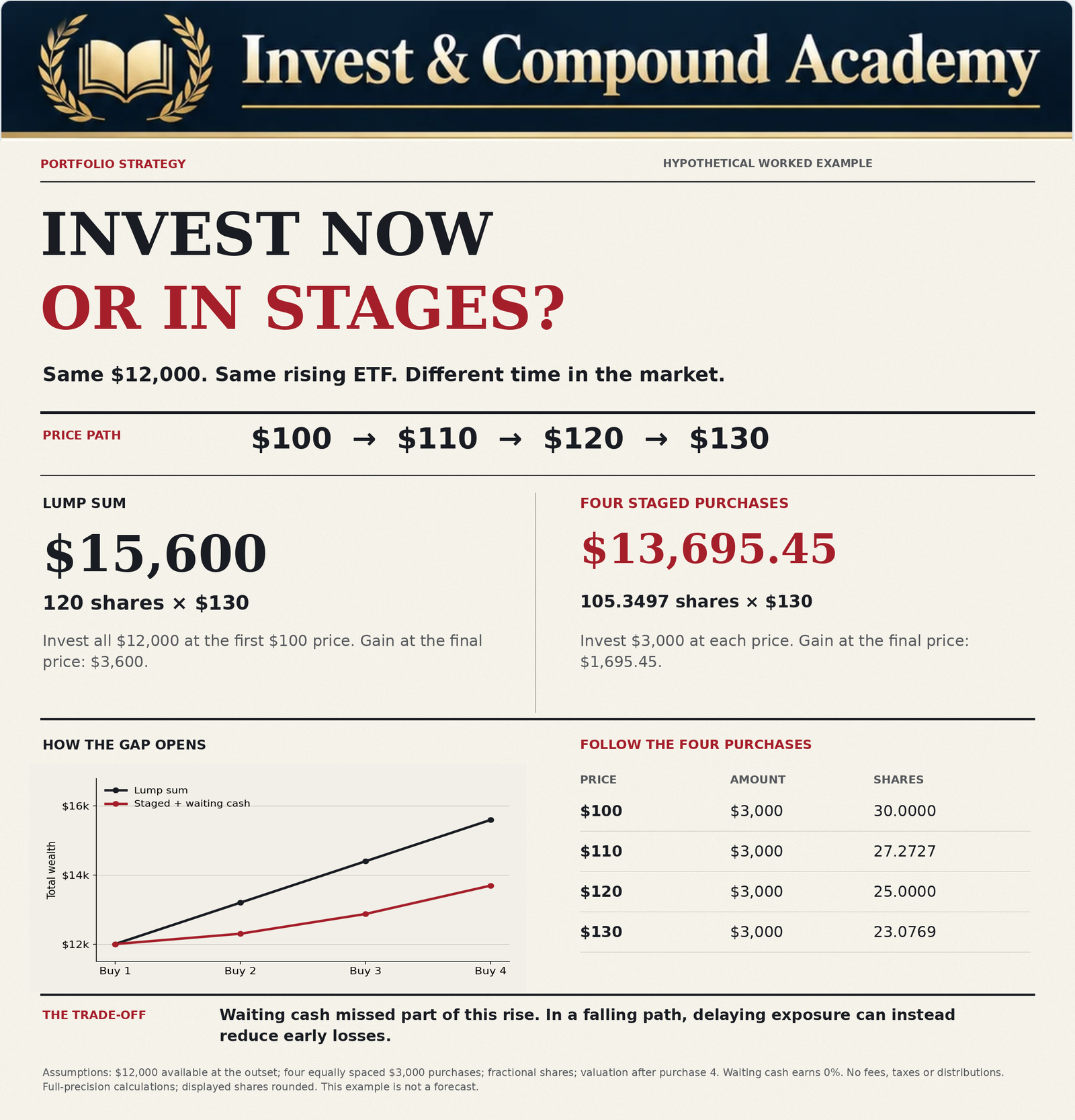
Numerical examples make the differences between immediate and staged investing easier to understand. Consider an investor with $12,000 available. The investor intends to purchase a hypothetical diversified ETF. Two strategies are compared. Under lump-sum investing, all $12,000 is invested at the first observation date. Under staged investing, $3,000 is invested at each of four monthly observation dates. Assume fractional shares are available. Ignore distributions, taxes, trading costs and interest on uninvested cash for this first comparison.
Rising Market Assumptions
| Purchase date | ETF price |
|---|---|
| Month 1 | $100 |
| Month 2 | $110 |
| Month 3 | $120 |
| Month 4 | $130 |
Lump-Sum Outcome
The investor purchases: $12,000 ÷ $100 = 120 shares. At the final price of $130, the shares are worth: 120 × $130 = $15,600. The investment gain is $3,600, or 30%.
Staged-Investment Outcome
The investor makes four purchases:
| Month | Contribution | Price | Shares acquired |
|---|---|---|---|
| 1 | $3,000 | $100 | 30.0000 |
| 2 | $3,000 | $110 | 27.2727 |
| 3 | $3,000 | $120 | 25.0000 |
| 4 | $3,000 | $130 | 23.0769 |
| Total | $12,000 | 105.3497 |
At $130 per share, the position is worth approximately $13,695.45. The staged strategy produces an investment gain of approximately $1,695.45.
Why Lump Sum Won
The difference is not caused by a special compounding trick. The immediate investor purchased more shares at the initial price. Every share participated in the subsequent advance. The staged investor purchased fewer shares as prices increased. The approximately $1,904.55 difference in ending wealth reflects the consequence of delayed exposure in this hypothetical market.
Scenario Analysis: A Market That Falls
Now suppose the ETF declines over the same period. The purchase dates remain unchanged.
Falling Market Assumptions
| Purchase date | ETF price |
|---|---|
| Month 1 | $100 |
| Month 2 | $90 |
| Month 3 | $80 |
| Month 4 | $70 |
Lump-Sum Outcome
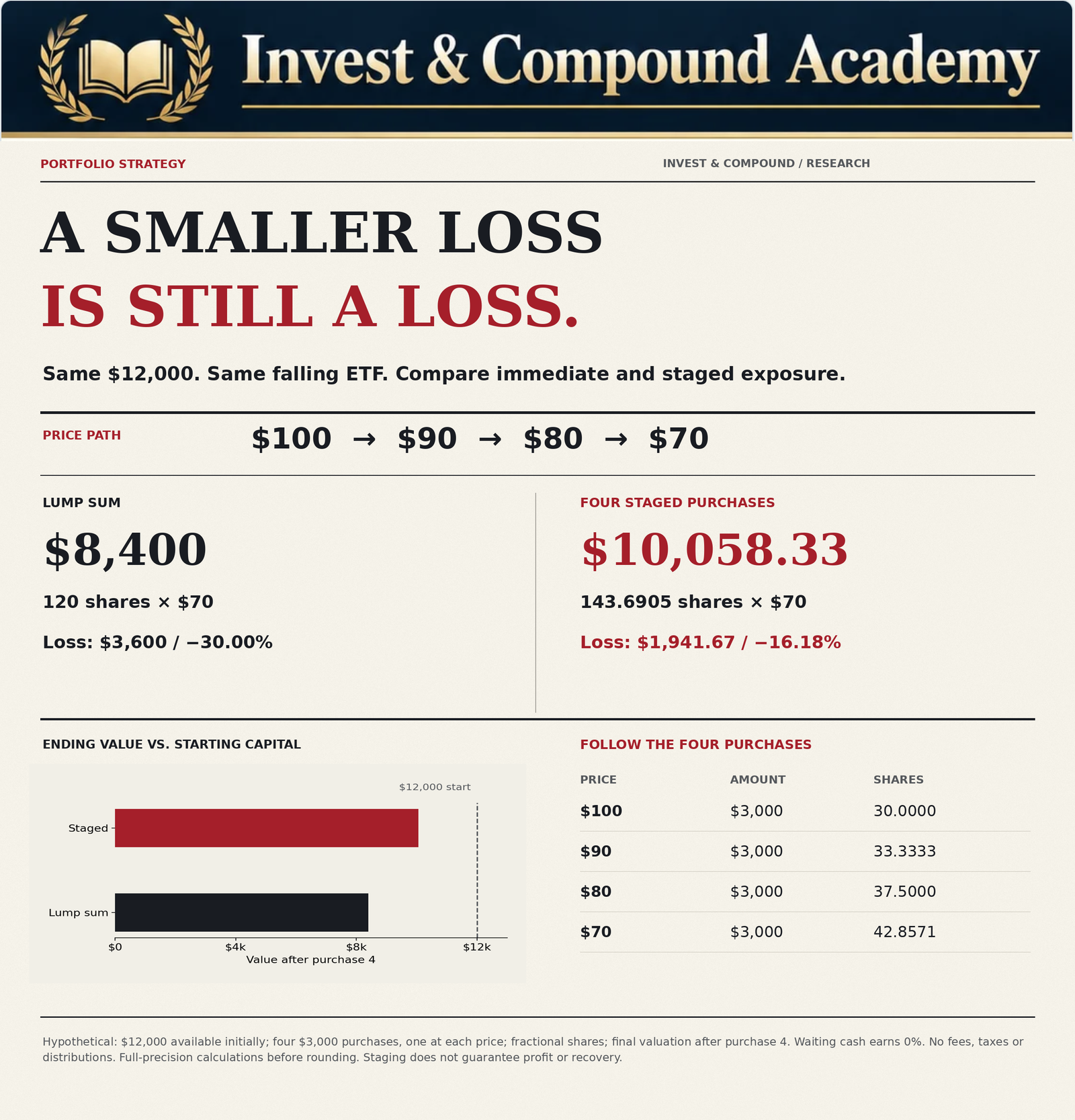
The lump-sum investor purchases 120 shares at $100. At the final price of $70, the position is worth: 120 × $70 = $8,400. The investor has an unrealized loss of $3,600, or 30%.
Staged-Investment Outcome
The staged investor purchases:
| Month | Contribution | Price | Shares acquired |
|---|---|---|---|
| 1 | $3,000 | $100 | 30.0000 |
| 2 | $3,000 | $90 | 33.3333 |
| 3 | $3,000 | $80 | 37.5000 |
| 4 | $3,000 | $70 | 42.8571 |
| Total | $12,000 | 143.6905 |
At the final price of $70, the shares are worth approximately $10,058.33. The staged investor experiences a loss of approximately $1,941.67.
Why Staged Investing Won
Some capital remained in cash while the market was falling. Later contributions purchased shares at lower prices. By the end of the period, the staged investor owned more shares than the lump-sum investor. The staged strategy therefore suffered a smaller loss.
The Important Limitation
Both investors lost money. Gradual deployment reduced the decline but did not eliminate it. If the ETF continued falling after the final purchase, the staged investor would then be fully exposed to the additional losses. Once the capital has been deployed, the portfolio’s future market risk depends on the assets held, not the original purchase schedule.
Scenario Analysis: A Sideways Market
Now consider a market that trades at the same price on all four purchase dates. The ETF price remains $100. The lump-sum investor purchases 120 shares at the beginning. The staged investor purchases 30 shares on each of four dates, also accumulating 120 shares. At the final price of $100, both positions are worth $12,000. Neither strategy gains an advantage from the share-price path. However, the staged investor may earn interest on temporarily uninvested cash. Alternatively, repeated transaction costs may reduce the staged result.
The net outcome therefore depends on the assumptions.
What the Three Scenarios Demonstrate
| Market path | Lump-sum final equity value | Staged final equity value | Better result |
|---|---|---|---|
| Rising: $100 to $130 | $15,600 | Approximately $13,695 | Lump sum |
| Falling: $100 to $70 | $8,400 | Approximately $10,058 | Staged |
| Flat: $100 throughout | $12,000 | $12,000 | Equal before other costs |
These are deliberately simplified examples. They demonstrate how different market paths produce different outcomes. They do not identify which path is most likely in the next four observation dates. The purpose of the comparison is to understand the trade-off, not to claim a forecast.
Why the Sequence of Returns Matters
The total movement between the initial and final market prices does not always describe the complete investment outcome. For a staged investor, prices on intermediate purchase dates determine the number of shares acquired. Two markets can begin at $100 and finish at $110 but produce different staged-investment returns.
Path A: Initial Decline Followed by Recovery
Assume prices of $100, $80, $90 and $110. The staged investor purchases more shares during the lower-price months. Four $3,000 purchases on Path A acquire approximately 128.1061 shares, worth $14,091.67 at the final $110 price.
Path B: Initial Rally Followed by Decline
Assume prices of $100, $125, $120 and $110. The staged investor purchases fewer shares during the expensive middle months. Path B acquires approximately 106.2727 shares, worth $11,690 at the final $110 price. The lump-sum position is $13,200 in either path, before other cash flows or costs. Both paths finish at $110. But the staged investor accumulates different quantities of shares.
Why Intermediate Prices Matter
For equal dollar contributions, the number of shares acquired is:
Ending value then equals:
This makes the staged strategy path-dependent. The immediate investor’s share count is determined by the initial price alone, assuming no later changes or distributions. The staged investor’s share count depends on multiple purchase prices.
Why This Matters for Backtesting
A reliable historical comparison must use actual purchase-date observations rather than just beginning and ending index values. It should also account for distributions, cash returns, fees and the selected investment horizon. A simplified comparison using only annual price changes may miss important differences between deployment strategies.
How Interest Earned on Cash Changes the Result
Earlier examples assumed that uninvested cash earned no interest. In reality, money awaiting investment might be held in a savings account, money-market fund or short-term government securities. This can reduce the opportunity cost of staged investing. However, cash yields change over time. They may also differ across currencies, financial institutions and account types.
A Simplified Interest Example
Suppose an investor has $12,000. The investor follows a four-purchase monthly deployment schedule: $3,000 initially, followed by three monthly investments of $3,000. Assume the remaining cash earns an effective annual return of 4%. A corresponding effective monthly rate is:
This equals approximately 0.3274%. If the investor keeps the cash interest rather than adding it to the scheduled purchases, the temporary balances can earn a modest amount during the deployment period.
With purchases at time zero and months one, two and three, apply the effective monthly cash return before each subsequent purchase. Deduct the scheduled $3,000 from the cash account each time and retain interest as cash. Under these assumptions, $59.18 of cash interest remains immediately after the fourth purchase. A rising-path staged balance becomes $13,695.45 of shares plus $59.18 of cash, or $13,754.64 using full-precision calculations. Actual interest-crediting conventions, rates and tax treatment can differ.
Why Cash Interest Does Not Eliminate Opportunity Cost
Cash returns improve the staged strategy relative to holding idle, non-interest-bearing cash. But they do not necessarily match the return of the intended investment. If the ETF appreciates substantially, a 4% annualized cash yield for a few months may compensate for only a small fraction of the missed equity gain. Conversely, during a market decline, cash interest can improve the staged strategy’s relative result.
The Role of Inflation
A positive nominal cash yield does not necessarily produce a positive real return. If inflation exceeds the after-tax cash return, temporarily uninvested capital may lose purchasing power. The appropriate comparison should therefore consider nominal investment returns, cash interest, fees, taxes and inflation when relevant.
How the Deployment Period Influences Results
One of the most consequential decisions in staged investing is how long to spread out the capital. An investor could deploy a lump sum over one month, three months, six months, twelve months or longer. Longer periods increase the amount of time during which some capital remains outside the intended investment.
Short Deployment Periods
A relatively short schedule reduces the length of delayed exposure. It also provides less opportunity to purchase shares across a prolonged decline.
Long Deployment Periods
A longer schedule can reduce immediate exposure for a greater period. However, it also creates more opportunity cost when markets rise. Vanguard’s research emphasizes that longer cost-averaging periods generally increase the relative disadvantage associated with delayed exposure when risk assets provide positive expected returns.
No Universally Optimal Number of Months
It would be misleading to recommend three months as universally superior to six months. The right schedule depends on the investor’s reasons for staging, the cash alternative, asset allocation and tolerance for short-term losses. If an investor chooses staged investing for behavioral reasons, a predetermined completion date is particularly important. Without a completion rule, a temporary strategy can become indefinite market avoidance.
Does Staged Investing Reduce Risk?
The answer depends on which risk is being measured and over what period. At the beginning of staged deployment, the investor holds less exposure to the intended risky asset. That generally reduces the immediate sensitivity of the total available capital to movements in that asset. However, it does not eliminate the risk of losing money.
Temporary Equity Exposure
Suppose an investor intends to allocate $100,000 to equities. Under immediate deployment, the full amount is exposed. Under a staged strategy, the first purchase might involve only $25,000, with $75,000 temporarily held in cash. If equities decline 20% immediately and cash remains unchanged, the immediate investor loses $20,000. The staged investor’s existing equity position loses $5,000. That illustrates a genuine temporary reduction in downside exposure.
The Cost of Reduced Exposure
If equities instead rise 20%, the immediate investor gains $20,000. The staged investor’s equity holdings gain only $5,000, before considering subsequent purchases or cash earnings. Reduced exposure protects against some losses and reduces participation in some gains.
Once Fully Invested
After both investors hold the same asset allocation, their future market sensitivity may become similar, even though their accumulated portfolio values and share quantities differ. The staged strategy does not permanently transform a risky investment into a safe one.
Risk Capacity Versus Risk Tolerance
Risk capacity concerns the financial ability to withstand losses. Risk tolerance concerns willingness to accept uncertainty and volatility. An investor with sufficient long-term capital but substantial emotional discomfort may prefer gradual deployment. An investor who cannot afford a market decline may need a different asset allocation rather than merely a slower schedule. These are not the same problem.
Review the bear-market guide, correction-duration research and bear-market recovery history before assuming a staged purchase schedule gives losses a deadline. A household’s liquidity needs can outlast—or arrive before—a market recovery.
Investor Behavior and the Cost of Regret
Financial decisions are influenced by psychology. A large investment made immediately before a market decline can create intense regret. An investor may begin questioning the decision even when the original investment horizon was twenty years. This can encourage unnecessary selling.
Loss Aversion
Loss aversion refers to the tendency for losses to carry greater psychological weight than equivalent gains for many people. A 20% market decline may feel more significant than an earlier 20% gain. The investor’s response can affect whether the planned strategy is maintained.
The Appeal of Multiple Entry Dates
Staged investing reduces dependence on one purchase date. The investor knows that some later contributions may occur at lower prices if markets decline. That can provide emotional comfort. However, multiple purchases do not remove uncertainty. They distribute entry timing over a period.
Regret Has Two Directions
An investor may regret investing immediately before a market decline. Another investor may regret delaying investment while markets rise. A realistic decision framework should consider both.
Avoiding a Behavioral Failure
If a gradual schedule helps an investor enter an appropriate portfolio that would otherwise remain entirely unfunded, it may have practical value. But the schedule must be followed. An investor who repeatedly postpones later contributions whenever markets appear expensive may not actually complete the investment. That defeats the purpose of establishing a predetermined plan.
Is a Hybrid Strategy Reasonable?
Some investors choose to invest part of an available sum immediately and stage the remainder. This combines aspects of both approaches. For example, an investor with $40,000 might invest $20,000 immediately and divide the other $20,000 into four $5,000 purchases at months one, two, three and four. The immediate purchase occurs at time zero; uninvested capital remains in cash between installments.
Potential Advantages
The immediate portion participates fully if markets rise. The delayed portion can be invested at lower prices if markets decline during the schedule. The strategy may also be psychologically easier for some investors.
Limitations
The hybrid strategy does not eliminate the basic trade-off. It still holds some capital outside the intended investment temporarily. It can underperform full immediate deployment in rising markets and full delayed deployment in particular falling-market paths. There is no universal proof that a 50/50 hybrid provides the best financial outcome.
Avoid Choosing Percentages Arbitrarily
A hybrid structure should be selected for a reason. The investor might want to limit the immediate loss exposure associated with a large financial windfall. Or the investor might need time to complete operational steps while maintaining partial market participation. A precise 50/50 split should not be treated as inherently optimal without supporting analysis.
Market Corrections: Should You Invest Everything After a 10% Drop?
A market correction is conventionally a decline of at least 10% from a recent high. Investors sometimes interpret the correction threshold as an automatic opportunity to invest a lump sum. However, the fact that prices have fallen does not establish that the decline has ended.
The Risk of Further Losses
Suppose an ETF falls from $100 to $90. An investor purchases immediately at $90. The ETF subsequently declines to $72. The investor experiences a 20% loss from the purchase price. The initial correction did not identify the final market low.
The Risk of Waiting
Now suppose the ETF rebounds rapidly from $90 to $105. An investor waiting for a lower entry price may be forced to buy at a higher price or remain in cash. Neither outcome can be known in advance.
Lump Sum After a Correction
Investing immediately after a correction may be suitable when the investor has available long-term capital and the selected allocation remains appropriate. The case should rest on portfolio objectives and expected returns rather than the belief that a 10% decline reliably identifies a bottom.
Staged Buying During a Correction
A predetermined staged schedule can reduce initial exposure if prices continue falling. However, it can sacrifice upside if recovery begins immediately. The decision remains the same fundamental trade-off present under ordinary market conditions. A correction changes the starting price and economic environment, but it does not eliminate uncertainty.
The market-correction pillar defines the threshold, and correction versus bear market distinguishes severity. Buying during a correction and what to do during a correction examine the practical decisions without treating a percentage decline as a buy signal.
What About Investing at Market All-Time Highs?
Many investors hesitate to commit a large sum when stock indexes are near record levels. The concern is understandable: a decline may follow immediately. However, an all-time high is not automatically evidence of overvaluation. A growing economy and increasing corporate profits can support new nominal index highs over time.
Market Level Versus Valuation
A market trading at a record index level may be fairly priced relative to future earnings. Conversely, a market below its previous high may remain expensive if expected profitability deteriorates. The price index alone does not provide a complete valuation judgment.
The Cost of Waiting for a Pullback
Suppose the index is at 100. An investor waits for a 10% decline. The index rises to 140 before falling 10% to 126. The eventual purchase price after the correction is still 26% higher than the original level. This illustrates why waiting for a correction does not guarantee a better entry price.
Market Timing Requires Multiple Successful Decisions
An investor attempting to delay purchase must decide when to remain in cash and when to enter. If the intended investment then declines, another decision may be required. The process can become an indefinite sequence of forecasts. A predetermined investment method reduces dependence on continuous market prediction.
Our P/E ratio guide separates market price from earnings; the PEG ratio guide adds the uncertainty of growth forecasts. Market warning signs provides risk context, not a reliable calendar for deploying a lump sum.
Portfolio Allocation Is More Important Than Deployment Style
Before deciding whether to invest immediately or gradually, the investor should determine how much capital belongs in risky assets. A person with a near-term financial obligation may not be suitable for substantial equity exposure regardless of the deployment method.
A Retirement Portfolio Example
Suppose an investor has $80,000 available for long-term retirement investing. The intended portfolio is 70% diversified equities and 30% high-quality bonds. The allocation implies: $56,000 in equities. $24,000 in bonds. The immediate-versus-staged decision concerns the timing of this selected portfolio exposure. It does not require investing all $80,000 into one equity fund.
Staging the Entire Allocation
An investor could deploy the chosen 70/30 allocation gradually. Each installment would follow the intended asset weights.
Staging Only Equities
Alternatively, an investor might establish the bond allocation immediately and stage the equity allocation. That produces a different temporary risk profile. The portfolio’s initial allocation may be much more conservative than its intended long-term structure.
Why the Distinction Matters
Two staged strategies using the same total amount and deployment period can have different market exposures. A rigorous comparison should identify which assets are purchased at each stage and where unused cash is held. Without those details, the expression dollar-cost averaging is too vague to support a precise performance comparison.
Begin with building an ETF portfolio, then use the portfolio-maintenance workbook for subsequent review. The examples in VOO and VTI overlap and VOO versus QQQ show why underlying exposure matters more than the number of purchases.
Lump-Sum Investing in ETFs
Exchange-traded funds are commonly used for lump-sum investments because one purchase can establish exposure to a diversified portfolio. However, the chosen ETF matters.
Broad-Market ETFs
A broad equity ETF may provide exposure to a large group of companies. It remains vulnerable to systematic market declines.
International ETFs
International funds introduce foreign-market and potentially currency-related risks.
Bond ETFs
Bond funds carry interest-rate and credit risks. The effect of staging purchases depends on changes in bond prices and yields.
Dividend ETFs
Dividend-focused ETFs may provide distributions, but income does not eliminate capital risk.
Covered-Call ETFs
Covered-call funds have return profiles influenced by underlying securities and options strategies. Some sacrifice upside participation in exchange for premiums. The immediate-versus-staged comparison should therefore consider the actual fund strategy, not merely the fact that the product is an ETF.
Leveraged ETFs
Leveraged and inverse funds can have daily objectives and complex multiday compounding effects. The risks of deploying capital into them differ materially from ordinary diversified long-term equity investing. A recurring purchase schedule does not eliminate those structural risks.
For product fundamentals, see the ETF beginner’s guide and how ETFs work. SCHD, JEPI, JEPQ, SPYI and QQQI pursue different mandates. Use the ETF research guide to examine those differences before comparing purchase schedules.
Individual Stocks and the Risk of Averaging Into a Deteriorating Business
Staged investing into a diversified portfolio differs from repeated purchases of one declining company. An individual company’s share price may fall because of deteriorating earnings, excessive debt, competitive problems or financial distress. Purchasing additional shares simply because the price has declined can increase permanent-loss exposure.
A Value-Trap Example
Suppose a company’s stock initially trades at $100. The investor buys shares. The price falls to $70, and the investor purchases more. Later, expected earnings decline sharply. The stock falls to $40. The investor’s average acquisition cost has declined. But the fundamental investment thesis may have become weaker.
Why Lower Cost Is Not Enough
Average cost is an accounting measurement. It does not establish intrinsic value. A financially impaired company may never recover the earlier market price.
Periodic Fundamental Review
Investors should reassess financial statements, debt, cash generation and competitive position before committing additional capital to individual stocks. A scheduled purchase plan is not a substitute for understanding the investment.
The ETF versus stock guide compares pooled and company-specific exposure. Our stock-research guide helps organize the business questions that a lower average cost cannot answer.
Transaction Costs and Practical Implementation
Theoretical comparisons often ignore brokerage fees. Actual investors may face commissions, bid-ask spreads, foreign-exchange costs and account-specific restrictions. These costs can influence the relative attractiveness of a staged strategy.
Commission Example
Suppose an investor has $12,000. One lump-sum ETF purchase costs a $5 commission. A four-purchase staged strategy incurs four commissions of $5 each. The lump-sum commission is $5. The staged commissions total $20. The additional $15 may be small relative to the investment amount, but the effect increases when transaction costs are large relative to purchases.
Bid-Ask Spreads
Even commission-free ETFs may incur trading costs through bid-ask spreads. Repeated purchases can generate repeated spread costs. However, dividing the same total purchase value into installments does not automatically multiply proportional spread costs: the spread, order size and execution price on each date determine the actual expense.
Currency Conversion
An investor purchasing securities in another currency may incur conversion expenses. For a Canadian investor using a Canadian-dollar account to buy U.S.-listed ETFs, the cost depends on the brokerage’s currency arrangements and execution method.
Whole-Share Restrictions
Some accounts permit only whole-share purchases. That can prevent an investor from committing the exact scheduled amount at each date. Unspent cash may accumulate between purchases. A comparison should account for the actual number of shares purchased and any remaining cash.
Automatic Investment Features
Some brokerages support recurring ETF purchases. Others require manual orders. Available features can affect the operational convenience of different deployment strategies. A method that is difficult to implement consistently may produce greater behavioral or execution risk.
The ETF creation and redemption guide explains spreads and NAV. Whole-share ETF rebalancing covers rounding and residual cash, while the QQQ-to-QQQM switching analysis connects recurring fee savings with one-time execution costs.
Taxes and Account Structure
Tax consequences depend on jurisdiction, account type, investment and transaction history. The act of purchasing securities generally differs from selling them for a realized gain or loss. However, staged purchases can produce multiple acquisition dates and potentially different cost-basis records.
Taxable Accounts
Investors may need to track acquisition costs and subsequent adjustments. If portions of a position are sold later, the applicable tax treatment depends on jurisdictional rules.
Canadian Accounts
Registered accounts such as RRSPs and TFSAs have different tax treatments from nonregistered brokerage accounts. A purchase strategy should be evaluated alongside contribution eligibility and account rules.
U.S. Accounts
IRAs and employer-sponsored plans also operate under account-specific rules. Taxable investment accounts may involve capital gains, distributions and other reporting considerations.
Why Tax Considerations Should Not Dominate Everything
Tax efficiency matters for after-tax returns. But an investor should not purchase an unsuitable security solely because an account offers tax advantages. The underlying investment risk remains.
Our ETF versus mutual fund guide discusses wrapper differences. The mutual-fund-to-ETF switching workbook provides a separate cost framework when creating the lump sum itself would require selling an existing investment.
Cash Reserves Must Be Separated From Investment Capital
One of the most important practical distinctions is between money available for long-term investing and money required for financial stability. An investor may hold $70,000 in a bank account but need $20,000 for emergency reserves and $15,000 for a planned obligation. Only the remaining $35,000 may be suitable for discretionary long-term investment under the investor’s circumstances. The immediate-versus-staged question should apply to that $35,000, not automatically to the entire bank balance.
Why This Matters
Investing emergency reserves immediately does not become appropriate merely because historical research favors lump-sum deployment for suitable investment capital. The research compares strategies for money intended to be invested. It does not establish that essential liquidity should be placed into volatile assets.
Near-Term Financial Goals
Capital required for a home purchase, tuition payment, tax liability or essential expense may require a different risk approach. A short deployment schedule does not solve the problem of an unsuitable long-term asset for a near-term liability.
Long-Term Capital
Money genuinely intended for many years of investment can be evaluated differently. The investor may have greater flexibility to tolerate temporary losses, provided overall financial circumstances support that risk.
The Role of Inflation and Real Returns
The investment decision should also be evaluated in purchasing-power terms. Holding cash during the deployment period may earn interest. However, its real return depends on inflation and taxes.
Nominal Versus Real Return
The exact real return is:
Suppose cash earns 3% annually while inflation is 4%. The real return is: 1.03 ÷ 1.04 − 1 = approximately −0.96%. Purchasing power declines even though the nominal cash balance grows.
Why This Matters for Staged Investing
A short period of cash holding may involve only a modest purchasing-power effect. A long delay can compound the difference. However, equities can also experience negative real returns, particularly over shorter horizons. The real-return calculation does not automatically favor one strategy in every scenario. It simply provides a more complete measure of economic performance.
The inflation and investing pillar explains purchasing power. Dividend yield versus total return and dividend yield explained help avoid counting distributions twice. For income-fund accounting, see covered-call ETF financial reports.
Comparing Strategies Over Longer Investment Horizons
If both strategies eventually acquire the same portfolio, the initial deployment period may represent only a small part of a twenty- or thirty-year investment horizon. However, the differences created during that period can continue affecting wealth because one investor may accumulate more shares or a different starting balance.
Compounding the Difference
Suppose two investors finish the deployment period with different portfolio values. If both subsequently earn the same percentage returns and make no further contributions or withdrawals, the absolute difference between their balances generally changes as those returns compound.
A Hypothetical Example
Investor A finishes the deployment period with $13,000. Investor B finishes with $12,500. Assume both subsequently earn a constant 6% annual return for ten years. Investor A’s future value is: $13,000 × 1.06^10 ≈ $23,281. Investor B’s future value is: $12,500 × 1.06^10 ≈ $22,386. The initial $500 difference becomes approximately $895. These are hypothetical results and exclude fees, taxes and inflation.
The Economic Interpretation
An early difference in shares or portfolio value can persist. However, the example does not prove that lump sum will produce the larger initial balance. That depends on the deployment-period market path.
What If the Investor Is Approaching Retirement?
An investor close to retirement may have different financial priorities from someone decades away from needing the money. Large short-term losses can be particularly consequential when portfolio withdrawals will begin soon. However, simply spreading a purchase over several months does not necessarily address the full problem.
Sequence-of-Returns Risk
If an investor plans to withdraw capital shortly, a market decline can reduce the portfolio balance before or during withdrawals. Selling assets at depressed values may reduce participation in a subsequent recovery.
Asset Allocation First
An investor with imminent spending needs may require a portfolio containing sufficient lower-volatility or liquid assets. The allocation should be established before choosing the purchase schedule.
Staged Deployment as Behavioral Support
A gradual schedule may make a transition into a suitable portfolio easier. However, it should not be mistaken for a substitute for prudent retirement planning.
The Importance of Spending Reserves
Financial flexibility may be more important than predicting an optimal investment date. Investors should evaluate how essential expenses will be funded during unfavorable market conditions.
The compounding-with-withdrawals workbook examines the separate risk created by spending during an investment path. Purchase staging and withdrawal planning should not be treated as interchangeable.
Comparing the Decision Across Investor Profiles
The same capital-deployment question can produce different reasonable conclusions for different investors.
The Long-Term Investor With Stable Finances
An investor has $30,000 available, adequate emergency savings, no urgent spending obligations and a twenty-five-year investment horizon. The investor has already chosen a suitable diversified portfolio. Immediate investment may be attractive because it maximizes expected market exposure from the beginning. However, losses remain possible.
The Highly Loss-Averse Investor
Another investor has $30,000 available and the same long-term objective but fears a substantial immediate decline. The investor may be tempted to avoid investing indefinitely. A short staged schedule could help implement the intended allocation. The potential behavioral advantage comes with the opportunity cost of delayed exposure.
The Investor With Uncertain Employment
A third investor has $30,000 but faces significant income uncertainty. The relevant question is whether the money is genuinely available for long-term investing. Maintaining liquidity may be more appropriate than either strategy until the financial situation is clearer.
The Investor With Excessive Equity Concentration
A fourth investor already has substantial equity exposure. Adding another lump sum entirely to a concentrated sector could make portfolio risk excessive. The investor should address allocation and concentration before deciding how quickly to purchase.
The Retiree Funding Near-Term Withdrawals
A fifth investor needs capital for expenses during the next year. The immediate-versus-staged debate may be secondary to ensuring that near-term liabilities are funded appropriately. The examples demonstrate why a universal instruction is insufficient.
An economic recession can affect income and liquidity at the same time as asset prices. Historical corrections, correction frequency and S&P 500 correction statistics provide context; none establishes the next favorable purchase date.
An Investor Decision Framework
A useful decision process can be organized around several questions.
Is the Capital Actually Available?
Determine whether the amount has already been received or will arrive gradually through future income. If the money has not yet been earned, immediate deployment of the entire future contribution amount may not be possible.
Is the Capital Suitable for Long-Term Investment?
Exclude emergency reserves and money required for near-term obligations.
Has the Target Asset Allocation Been Established?
Choose appropriate equity, bond and cash exposures before deciding when to deploy them.
Can the Investor Financially Withstand Immediate Losses?
Stress-test potential declines. Consider whether losses would interfere with important financial objectives.
Can the Investor Behaviorally Withstand Immediate Losses?
Evaluate the likelihood of panic-selling or abandoning the plan after a decline.
What Return Is Available on Waiting Cash?
Consider after-tax cash yields, inflation and account conditions.
What Costs Does Staging Create?
Include commissions, spreads, foreign-exchange costs and operational complexity.
What Is the Completion Rule?
If gradual deployment is chosen, specify dates, amounts and the conditions under which the schedule would legitimately change.
How Will Success Be Evaluated?
Measure the actual portfolio’s performance relative to its objectives, not merely whether the chosen entry dates happened to be favorable.
Why a Fixed Schedule Is Better Than an Indefinite Waiting Strategy
A staged strategy is most coherent when the schedule is predetermined. For example, an investor might decide to purchase 25% immediately and the remaining 75% in three equal monthly installments. The schedule is clear. The investor does not need to make a new market forecast before each purchase. By contrast, a plan to invest when the market feels safer has no defined completion condition.
The Problem With Waiting for Certainty
Market conditions rarely become completely certain. After a decline, investors may fear further losses. After a rally, they may fear buying too high. This can create perpetual delay.
A Completion Date
A defined schedule reduces the risk of remaining out of the market indefinitely. It also makes it easier to evaluate the strategy afterward.
Legitimate Reasons to Change the Schedule
Changes in financial circumstances, investment suitability or important new information about the underlying assets may justify reconsideration. However, routine market volatility alone should not automatically lead to repeated improvisation. The purpose of a predetermined schedule is to reduce dependence on short-term forecasts.
How to Compare the Strategies Fairly
An accurate performance comparison must keep the underlying investment allocation consistent. It must also measure all assets, including uninvested cash, rather than only the portion already deployed.
Include Cash Balances
During staged deployment, the investor owns a combination of securities and cash. Both should be included when calculating total wealth. Ignoring cash would make the strategy appear worse than it actually is during declines. Ignoring cash interest would also distort the result when short-term yields are meaningful.
Include Distributions
An ETF may pay dividends or other distributions. A total-return comparison should treat them consistently.
Include Transaction Costs
Repeated purchases may incur more commissions. Spread expenses should be calculated using the actual order values and execution conditions.
Define the End Date
Comparing strategies immediately after the final staged purchase answers a different question from measuring outcomes five years later.
Use the Same Portfolio
A lump-sum investment into a broad equity ETF should not be compared with staged purchases of a completely different strategy without acknowledging the change in asset exposure.
Avoid Hindsight Optimization
A historical comparison should not assume that an investor knew the future market low. Choosing the best possible purchase dates after examining the data does not represent an implementable forward-looking strategy.
The Mathematics Behind a Fair Comparison
A fair comparison starts with the same cash amount, the same investment, a specified set of dates and one common valuation date. During deployment, staged wealth includes both the investment and waiting cash.
A positive difference favors lump sum in that scenario. A negative difference favors staging. The first calculator below accepts four purchase prices; the second models a constant annual return and lets you change the number and spacing of installments. Both deduct the entered commission from the original capital rather than silently adding external money.
Common Mistakes When Comparing Lump Sum and DCA
Confusing Regular Salary Contributions With Delayed Investment
Investing new income as it arrives differs from holding back an existing lump sum.
Assuming Lump Sum Always Wins
Historical outperformance rates are not guarantees. A severe decline immediately after investment can make staged deployment preferable in that particular outcome.
Assuming Dollar-Cost Averaging Prevents Losses
A staged strategy can still lose substantial value.
Ignoring Uninvested Cash
Cash is part of staged-investment wealth until it is deployed.
Ignoring Cash Interest
Cash earnings can affect the result, particularly when rates are elevated or the deployment period is long.
Ignoring Transaction Costs
Frequent purchases may increase commissions. Proportional costs also depend on the amount purchased and prevailing spreads.
Comparing Different Investments
A change in underlying asset allocation can dominate differences caused by purchase timing.
Focusing Only on Average Cost Per Share
The objective is not necessarily to achieve the lowest average cost. It is to obtain a suitable risk-adjusted investment outcome.
Treating a Market Correction as a Guaranteed Opportunity
Prices can continue falling after reaching the conventional correction threshold.
Delaying Indefinitely
A staged strategy without a defined completion date can become unstructured market avoidance.
Using Emergency Reserves
Historical investing research does not justify putting essential liquidity into volatile assets.
Ignoring Investor Behavior
A strategy that appears mathematically attractive may fail in practice if the investor cannot tolerate its short-term consequences.
Frequently Asked Questions
Is Lump-Sum Investing Better Than Dollar-Cost Averaging?
Lump-sum investing has historically outperformed many common staged-investment approaches more often than not, but it does not win in every market environment. The appropriate choice depends on available capital, risk capacity and investor behavior.
What Percentage of the Time Does Lump Sum Win?
Vanguard’s 2023 research reported that immediate investment outperformed common cost-averaging strategies approximately two-thirds of the time. One global equity illustration found 68% outperformance using three equal purchases one month apart and a one-year outcome horizon.
Why Does Lump Sum Often Outperform?
Because capital invested sooner receives more exposure to assets with historically positive expected returns, rather than remaining temporarily in cash.
Can Dollar-Cost Averaging Outperform Lump Sum?
Yes. It can produce better results when prices decline sufficiently during the staged deployment period.
Does DCA Reduce Market Risk?
It temporarily reduces exposure to the intended risky asset while some capital remains in cash. It does not eliminate future risk once the funds are fully invested.
Is Dollar-Cost Averaging Safer?
It may reduce immediate downside exposure in a particular comparison, but safety depends on the assets, investment horizon, liquidity and financial situation.
Should I Invest All My Money at Once?
The amount available for long-term investing should first be separated from emergency reserves and near-term obligations. The appropriate deployment strategy then depends on the chosen portfolio and risk considerations.
Is It Better to Spread a Lump Sum Over Three or Twelve Months?
A longer schedule maintains more temporary cash exposure and may increase opportunity cost in rising markets. No deployment period is universally optimal.
Should I Wait for a Market Correction?
Waiting can result in buying at a lower price, but it may also mean missing gains or purchasing above today’s price after a later correction.
What If the Market Crashes Immediately After a Lump Sum?
The full investment experiences the applicable market loss. A staged strategy would generally have less initial equity exposure, but its future results depend on later purchase prices.
What If the Market Rises During DCA?
Later contributions purchase fewer shares, potentially reducing returns relative to immediate investment.
Does Cash Interest Make DCA Better?
Cash interest can improve staged-investment outcomes, but it does not guarantee that they will exceed lump-sum investing.
Does DCA Always Lower the Average Cost Per Share?
No. Its average cost depends on the purchase-price path. In steadily rising markets, later purchases occur at higher prices.
Can I Combine Lump Sum and DCA?
Yes. A hybrid approach invests some capital immediately and deploys the remainder gradually. It preserves some market exposure while retaining temporary cash.
Is a 50/50 Hybrid the Best Strategy?
Not universally. A 50/50 split may be a convenient compromise, but it is not mathematically optimal for every investor or market condition.
Does the Investment Horizon Matter?
Yes. Longer horizons affect the suitability of risky assets and the financial consequences of temporary declines. The entry strategy should be considered within the broader investment plan.
Should Retirees Use DCA?
The decision depends on liquidity, withdrawal needs, asset allocation and risk capacity. Gradual deployment alone does not solve sequence-of-returns risk.
Can ETFs Be Purchased Using Either Strategy?
Yes, subject to account capabilities, transaction costs and the characteristics of the ETF.
Does DCA Work for Individual Stocks?
Scheduled purchases are possible, but the strategy does not eliminate company-specific risk or prevent permanent losses.
How Are Taxes Affected?
The consequences depend on jurisdiction, account type, acquisition costs and later transactions. Multiple purchase dates may require more detailed cost-basis records.
What Is the Best Strategy for a Long-Term Investor?
There is no universally superior strategy for every investor. Research often favors immediate deployment of suitable long-term capital on expected-return grounds, while gradual investing may provide behavioral benefits in certain circumstances.
Choose the Trade-Off Before the Outcome Is Known
Lump-sum investing establishes the intended market exposure immediately. Staging retains temporary cash and spreads purchase prices across a defined period. Neither method removes the need for suitable investments, an appropriate allocation and adequate liquidity. The decision is most useful when it is made before the future path is visible. An immediate purchase can be followed by losses; a staged plan can miss an advance. Evaluate the choice against the assumptions and financial circumstances available at the time, rather than judging every decision by hindsight.
A written completion rule can help someone who stages existing cash for behavioral reasons. It should still allow a legitimate response to changing household finances or investment suitability. The goal is a workable capital-deployment process with understood costs and risks.
Lump-Sum Investing vs DCA Calculator: Four Purchase Prices
Reproduce the rising or falling example, or enter another sequence. The model keeps the starting capital equal and includes any retained cash interest.
Lump-Sum Investing Calculator: Timing and Waiting Cash
Change the schedule under a smooth assumed market return. A longer schedule changes both risky-asset exposure and the period during which cash can earn interest.
Explore the Earlier Academy Pillars
Connect lump-sum investing with the fifteen earlier pillars on market behavior, economics, fund structure and recurring contributions.
Continue Learning in the Invest & Compound Academy
Develop the contribution, allocation, execution and measurement questions that sit alongside a capital-deployment decision.
Capital deployment, investment risk and portfolio strategy
Market Correction Pillar | Indexes and Markets | Portfolio Construction
Sources and Further Reading
Reference review: October 18, 2026. The identified historical finding uses Vanguard’s stated Figure 2 assumptions. Vanguard is an investment manager and the author of that research; its reported historical frequencies are not guaranteed future probabilities. All other paths, cash rates and calculator defaults are hypothetical. Calculations use full precision before display rounding. No current market quotes or investment forecasts are provided.
- Vanguard Research: Cost Averaging — Invest Now or Temporarily Hold Your Cash? Megan Finlay and Josef Zorn, February 2023. Figure 2 and its methodology notes.
- FINRA: The Benefits and Limitations of Dollar-Cost Averaging, May 19, 2026. Existing cash, paycheck contributions, opportunity costs and transaction expenses.
- SEC Investor.gov: Dollar Cost Averaging — scheduled equal-amount purchases.
- SEC Investor.gov: Asset Allocation — objectives, time horizon and portfolio exposures.
- SEC Investor.gov: Mutual Fund and ETF Fees and Expenses — operating expenses and transaction costs.
This article provides general financial education, not personalized investment, financial, legal or tax advice or a recommendation to buy, sell or hold a security.
Lump-sum investing can expose more capital to immediate losses. Staged investing retains temporary cash and can miss gains. Neither method guarantees profits, capital protection, a favorable average purchase price or a particular recovery period. Historical research depends on its sample and assumptions.
Investments can lose principal permanently. Fees, taxes, distributions, currency effects, account rules, cash returns and personal liquidity needs affect outcomes. Diversification and asset allocation do not guarantee positive returns. Review current product documents and consider qualified professional advice where appropriate.

