$10,000 Investment Growth in 20 Years: Calculator and Examples
How much will $10,000 grow in 20 years? Compare return scenarios, monthly contributions, fees and inflation using transparent calculations.
How much will $10,000 grow in 20 years? At hypothetical constant effective annual returns of 5%, 7% and 10%, it becomes approximately $26,533, $38,697 and $67,275, respectively, before fees and taxes and with no new deposits. These are investment growth scenarios, not market forecasts. The balance changes substantially when monthly savings are added. At the same 7% effective annual return, an initial $10,000 plus $500 at each month-end reaches approximately $292,465. Of that amount, $130,000 was deposited; about $162,465 is modeled investment growth.
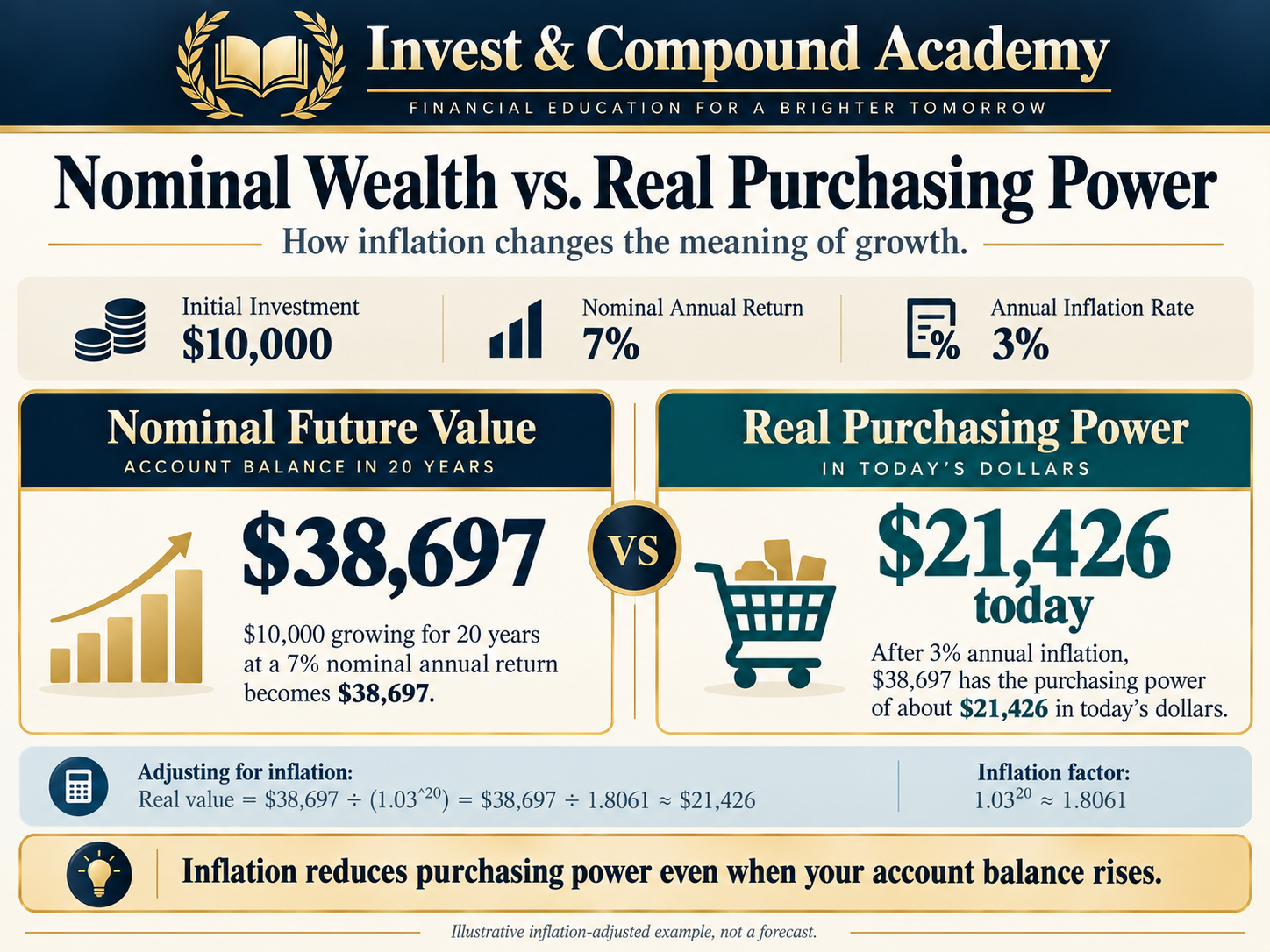
Purchasing power gives another perspective. The $38,697 lump-sum scenario is equivalent to approximately $21,426 today if inflation remains 3% annually. This guide compares the twenty-year outcomes directly, while our Rule of 72 calculator examines the separate question of doubling time.
Try the Investment Growth Calculator
How Much Can $10,000 Become in Twenty Years?
The future value of a one-time investment can be calculated using the compound-growth formula.
For a starting amount of $10,000 and a twenty-year horizon:
Where r represents the assumed effective annual growth rate expressed as a decimal. At 7%, r equals 0.07. The calculation becomes $10,000 × 1.07^20. The result is approximately $38,696.84. The initial $10,000 is included in that value. The hypothetical investment growth is approximately $28,696.84. No additional contributions are assumed.
Twenty-Year Growth Comparison
| Assumed annual return | Value after 20 years | Investment growth |
|---|---|---|
| 0% | $10,000 | $0 |
| 2% | $14,859 | $4,859 |
| 3% | $18,061 | $8,061 |
| 4% | $21,911 | $11,911 |
| 5% | $26,533 | $16,533 |
| 6% | $32,071 | $22,071 |
| 7% | $38,697 | $28,697 |
| 8% | $46,610 | $36,610 |
| 10% | $67,275 | $57,275 |
| 12% | $96,463 | $86,463 |
All values are rounded hypothetical projections using constant effective annual returns, no additional cash flows, and no taxes or investment fees. The table highlights two important relationships. First, the initial capital does not need to be large for compound growth to become economically meaningful. Second, long-run outcomes are highly sensitive to the rate of return. The challenge is that investors cannot know their future twenty-year returns in advance. A higher projected rate should not automatically be interpreted as a realistic or achievable return for a particular asset.
Understanding the Future-Value Formula
The mathematics of investment growth can appear complicated, but the core relationship is straightforward. At the end of each year, the portfolio’s value is multiplied by one plus that year’s return. Under a constant-return model, the same multiplication factor applies repeatedly.
First Year
Suppose the initial investment is $10,000 and the assumed annual return is 7%. After one year, $10,000 × 1.07 = $10,700. The investment has increased by $700.
Second Year
The next 7% return applies to the larger balance: $10,700 × 1.07 = $11,449. The second year’s hypothetical gain is $749. That is greater than the first year’s $700 gain.
Third Year
The calculation continues: $11,449 × 1.07 = $12,250.43. As long as gains remain invested, subsequent percentage returns apply to the accumulated balance. This process produces compound growth.
Why Exponents Appear in the Formula
Multiplying a balance by 1.07 twenty times is equivalent to multiplying by 1.07 raised to the twentieth power. That is why the general future-value formula contains an exponent representing the number of compounding periods. The exponent is responsible for much of the long-term sensitivity to the assumed rate. However, the formula describes a hypothetical path based on a specified constant return. Actual investments generate variable returns, including negative outcomes.
The compound-interest guide develops the underlying growth mechanics. How to measure investment growth explains the separate accounting for deposits, withdrawals and gains.
Simple Interest Versus Compound Growth
Simple interest and compound interest describe different mathematical processes. Under simple interest, the return is calculated only on the original principal. Under compound interest, previously accumulated returns can also earn additional returns.
Simple Interest Example
Suppose $10,000 earns simple interest of 7% annually for twenty years. The annual interest is $700. Over twenty years, total interest equals $14,000. The ending value is $24,000.
Compound Growth Example
At 7% annual compounding, $10,000 × 1.07^20 ≈ $38,697. The difference is substantial. The compound-growth model generates approximately $14,697 more than the simple-interest model.
Why This Distinction Matters
Investors commonly use the phrase compound interest to describe long-term stock-market growth. However, stock returns are not contractually fixed interest payments. For equities, the more precise concept is compounded investment return. The same mathematical relationships can describe a portfolio’s long-run growth, but actual results depend on market performance.
Reinvestment Is Important
An investor who withdraws returns as they are generated will generally experience a different wealth trajectory from an investor who leaves them invested. That does not make withdrawals inherently inappropriate. Retirees, for example, may need portfolio income for living expenses. It means that a future-value calculation must reflect whether cash remains invested or leaves the account.
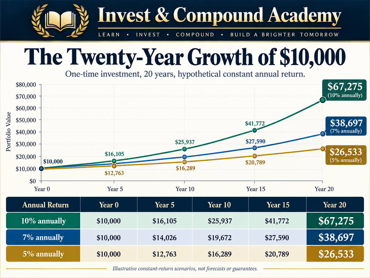
How $10,000 Grows at 5%, 7%, and 10%
Comparing several return assumptions helps reveal how compounding changes over time. Consider three hypothetical portfolios, all beginning with $10,000. Portfolio A earns 5% annually. Portfolio B earns 7%. Portfolio C earns 10%. Assume no contributions, withdrawals, fees, or taxes.
Growth Over Time
| Year | 5% annual return | 7% annual return | 10% annual return |
|---|---|---|---|
| 0 | $10,000 | $10,000 | $10,000 |
| 5 | $12,763 | $14,026 | $16,105 |
| 10 | $16,289 | $19,672 | $25,937 |
| 15 | $20,789 | $27,590 | $41,772 |
| 20 | $26,533 | $38,697 | $67,275 |
The differences are relatively modest during the early years. By Year 20, the 10% scenario produces a balance more than twice as large as the 5% scenario.
Why Growth Accelerates in Dollar Terms
Under a constant positive percentage return, each year’s gain is calculated on the previous year’s larger balance. The dollar increase therefore becomes larger even though the percentage rate remains unchanged.
Why Higher Growth Assumptions Require Caution
A 10% projection produces an attractive result. A 12% projection produces an even larger one. But the fact that a rate generates an appealing future value does not establish that investors can reasonably expect to earn it. Investment return assumptions should reflect the asset allocation, risks, valuation environment, fees, and uncertainty associated with the intended strategy. The appropriate process is to examine several possible outcomes rather than select the most attractive projection.
What Does a 7% Return Really Mean?
An assumed 7% annual return is commonly used in educational examples. However, the meaning of 7% depends on how it is defined. It might represent an assumed nominal return. It might represent an inflation-adjusted real return. It might describe a historical annualized rate. Or it might be a forward-looking planning assumption. These are not interchangeable.
Nominal Return
A nominal return measures the change in investment value in currency terms before adjusting for inflation. If a portfolio grows from $10,000 to $10,700, the nominal return is 7%.
Real Return
A real return adjusts for changes in purchasing power. If inflation during the same period is 3%, the exact real return is 1.07 ÷ 1.03 − 1 ≈ 3.88%.
Gross Versus Net Return
A gross return may describe performance before certain expenses. A net return incorporates specified costs. The investor’s actual account growth may also be affected by taxes, transaction costs, and other expenses.
Expected Versus Realized Return
An expected return is an assumption about future performance. A realized return describes what actually occurred. An investment can have a positive expected return while delivering a negative realized return over a particular period. For transparent financial planning, the term 7% return should always be accompanied by enough context to identify its meaning.
Why a Twenty-Year Investment Does Not Grow Smoothly
One of the largest limitations of compound-interest examples is the assumption that returns are constant. Financial markets rarely behave that way. A stock portfolio may rise 18% in one year, decline 22% in another, and recover over subsequent years. The long-term result depends on the compounded return factors. Without intervening cash flows, their order changes the path but not the terminal product. With deposits or withdrawals, the order can also change final wealth.
A Two-Year Example
Suppose a portfolio gains 20% in the first year and loses 20% in the second. Starting with $10,000, the balance becomes $12,000 after Year 1 and $9,600 after Year 2. The arithmetic average return is zero. But the compounded outcome is a 4% loss.
Why Average Returns Can Mislead
An arithmetic average does not fully describe wealth growth. For investment projections, the compound annual growth rate is a more relevant measure when evaluating how a starting balance changed into an ending balance without external cash flows.
Compound Annual Growth Rate
If a portfolio rises from $10,000 to $25,000 over twenty years, CAGR = (2.5)^(1/20) − 1, approximately 4.69% annually. The calculation identifies the constant annual rate equivalent to the observed total growth. It does not imply that the investment actually earned 4.69% every year.
Why Historical CAGR Is Not a Forecast
The historical performance of an index can help investors understand previous outcomes. However, future earnings, interest rates, valuations, economic conditions, and investor behavior will differ. No historical twenty-year result guarantees the next twenty-year return.
How Inflation Changes the Value of $10,000
Inflation changes purchasing power. An investment can generate a positive nominal return while providing much smaller real economic growth. The Bureau of Labor Statistics uses consumer price indexes to measure changes in consumer prices and explains how index ratios can translate nominal dollar values into purchasing-power comparisons. For long-term investment planning, a constant inflation assumption can provide a useful illustration.
A Twenty-Year Example
Suppose $10,000 grows at a hypothetical 7% nominal annual return for twenty years. The ending balance is approximately $38,697. Now assume inflation averages 3% annually. The inflation factor over twenty years is 1.03^20 ≈ 1.8061. Dividing the full-precision future balance by that factor gives approximately $21,426 in today’s purchasing power.
Interpreting the Result
The investor’s account would show approximately $38,697. But the amount would have purchasing power equivalent to about $21,426 today under the stated inflation assumption. This is not a loss in nominal value. It is the difference between nominal growth and real growth.
Why Personal Inflation May Differ
A national consumer price index measures changes across a representative basket of expenditures. Individual households may face different price changes because their spending patterns differ. Housing, health care, transportation, and other categories can account for different portions of household budgets. Therefore, a general inflation assumption is useful for planning but cannot perfectly represent every person’s future cost of living.
Our inflation and investing pillar examines purchasing power across asset classes. The economic recession guide addresses the separate issue of declining economic activity.
Twenty-Year Inflation Scenarios
Suppose a portfolio grows to $38,697 in nominal terms after twenty years. The real value depends on inflation.
| Assumed annual inflation | Purchasing power in today’s dollars |
|---|---|
| 0% | $38,697 |
| 2% | Approximately $26,042 |
| 3% | Approximately $21,426 |
| 4% | Approximately $17,661 |
| 5% | Approximately $14,584 |
These are hypothetical constant-inflation scenarios. The comparison demonstrates why investment goals should be defined in terms of future spending needs rather than only future account balances.
Future Cost of Living
The same calculation can be approached from the spending side. Suppose a household currently requires $50,000 annually to fund a particular standard of living. At 3% constant inflation, the equivalent nominal expense after twenty years would be approximately $90,306. A future balance that appears large relative to today’s income may support less spending than expected.
Why Investors Should Test Multiple Inflation Rates
A financial plan using only one inflation rate may underestimate uncertainty. Testing 2%, 3%, 4%, and 5% scenarios can show how sensitive the goal is to long-term purchasing-power changes. However, the scenario analysis should not imply that every inflation rate is equally likely. The purpose is sensitivity analysis, not an unsupported probability forecast.
What If You Add $100 Every Month?
A starting investment of $10,000 can grow through returns alone. Additional contributions create a second source of account growth. Suppose the investor adds $100 at the end of every month for twenty years. Assume a hypothetical 7% effective annual return. To calculate consistent monthly growth, convert the annual rate into an effective monthly rate:
At 7% annually, the monthly rate is approximately 0.5654%. The starting $10,000 compounds over 240 months. Each monthly contribution compounds from the date it is invested until the end of the period. The total ending value is approximately $89,450.
Separating Contributions From Growth
The investor contributes $10,000 initially and $100 × 240 months = $24,000 additionally. Total contributed capital is $34,000. The projected ending balance is approximately $89,450. The hypothetical investment growth is approximately $55,450. This distinction is essential. The future account balance reflects both new savings and investment returns. The full increase should not be described as investment performance.
What If You Add $250, $500, or $1,000 Monthly?
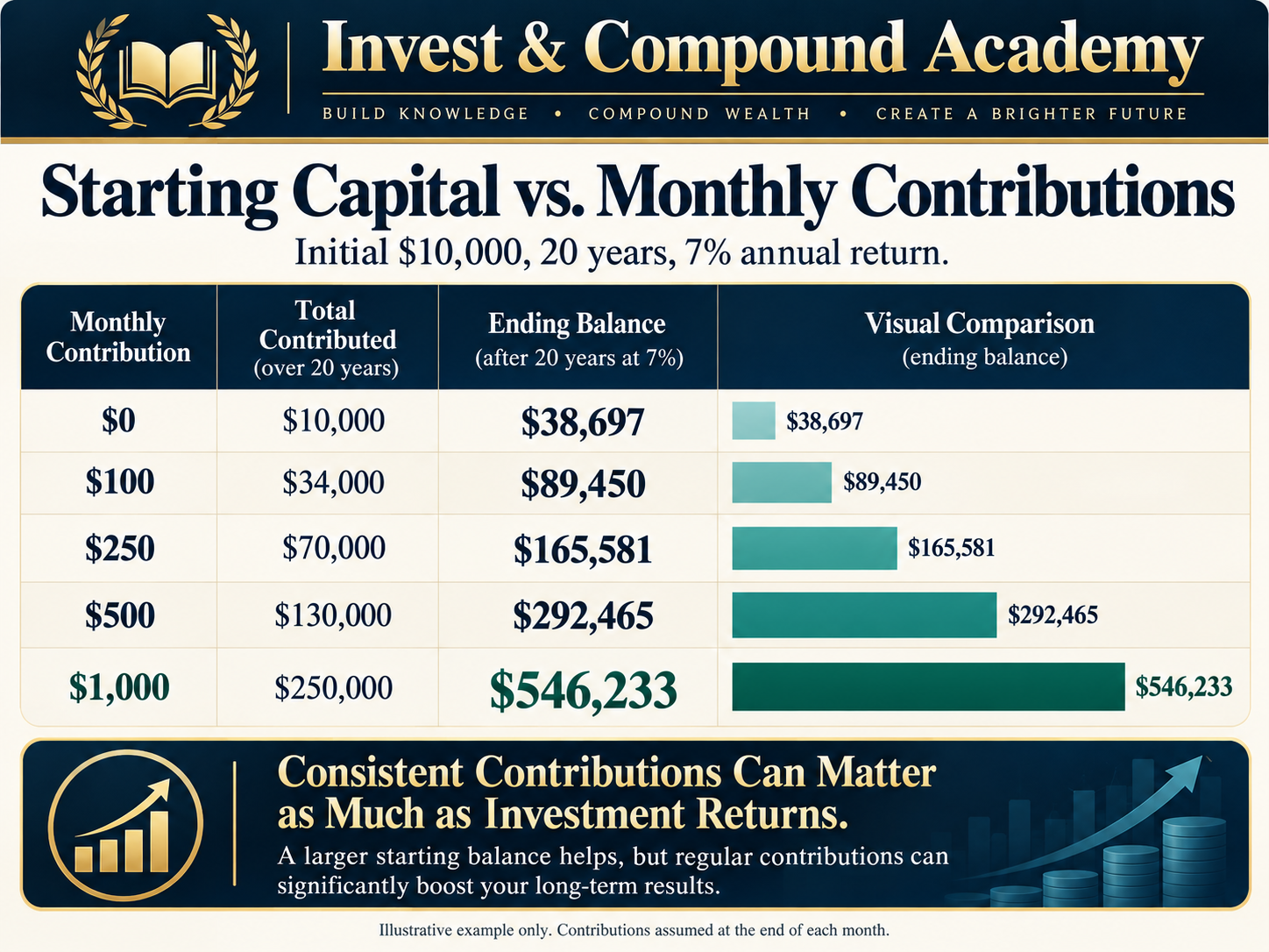
Regular contributions can have a larger effect than small adjustments to the expected return assumption. Consider four monthly contribution amounts. Each scenario begins with $10,000 and assumes a constant effective annual return of 7% over twenty years. Contributions occur at the end of each month.
| Monthly contribution | Total contributed over 20 years | Projected ending balance |
|---|---|---|
| $0 | $10,000 | $38,697 |
| $100 | $34,000 | $89,450 |
| $250 | $70,000 | $165,581 |
| $500 | $130,000 | $292,465 |
| $1,000 | $250,000 | $546,233 |
All amounts are rounded and exclude taxes and fees. The results show how regular saving can substantially increase an investor’s future account balance. However, larger contributions also require greater financial resources. An investor should not select a contribution amount based solely on the attractiveness of the projected result.
Affordability Matters
A contribution schedule should reflect household income, necessary expenses, emergency reserves, debt obligations, and other financial objectives. A smaller contribution maintained consistently may be more sustainable than an aggressive contribution that creates liquidity problems.
Contributions Must Be Distinguished From Investment Growth
An investor contributing $1,000 monthly over twenty years invests $240,000 beyond the initial $10,000. The large projected ending balance partly reflects that substantial saving effort. A responsible calculator should report principal and investment growth separately.
See dollar-cost averaging explained for purchase ledgers, average cost and recurring contributions. Here, the question is the twenty-year value of the complete account, including the starting $10,000.
How the Monthly Contribution Formula Works
The future value of a starting investment and fixed end-of-period contributions can be estimated with:
Here, P is the initial investment, C is the regular contribution, r is the effective return per contribution period and n is the number of periods. The first component represents growth of the starting amount. The second represents the accumulated value of recurring contributions.
Why Contribution Timing Matters
A contribution made at the beginning of a month has more time to earn returns than one made at the end. A calculator should specify whether contributions occur at the beginning or end of each period.
What Happens When the Return Is Zero?
If the periodic return is zero, the contribution component reduces to the total amount deposited. The future value is simply:
This special case avoids dividing by zero in a calculator.
What Happens When Returns Are Negative?
The standard constant-rate formula can calculate certain negative growth assumptions, provided the mathematical inputs remain valid. However, actual investment losses fluctuate rather than occurring at an identical rate each period. A professional financial tool should distinguish its deterministic assumptions from observed market performance.
How Investment Fees Reduce Long-Term Growth
Fees are one of the most important variables investors can evaluate before choosing an investment product. The SEC’s July 2025 investor bulletin explains that recurring fees reduce the amount of capital remaining in a portfolio to earn future returns. This creates a compounding effect.
A Twenty-Year Fee Example
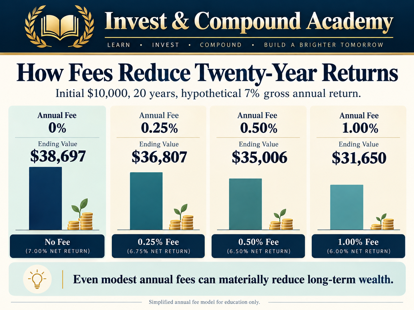
Suppose an investor starts with $10,000. Assume a hypothetical 7% effective annual gross return before an illustrative annual fee deduction. Under a simplified model, the portfolio first earns the gross return and then has a percentage-based fee applied to the resulting value. The annual multiplier is:
After twenty years:
Comparison
| Illustrative annual fee | Ending value after 20 years |
|---|---|
| 0% | $38,697 |
| 0.25% | $36,807 |
| 0.50% | $35,006 |
| 1.00% | $31,650 |
The resulting net effective annual growth assumptions are 7.0000%, 6.7325%, 6.4650% and 5.9300%, respectively. These values use a simplified annual fee model, not a precise simulation of fund-level daily expense accrual. For monthly contributions, the calculator converts the combined annual growth-and-fee factor to its equivalent monthly factor; it does not wait until December to charge a full annual fee on each new deposit. The differences become substantial over two decades.
At a 1% annual fee under the stated model, the ending value is approximately $7,046 lower than the no-fee scenario. This ending-wealth gap includes both fees deducted and the investment growth those dollars no longer earn; it is not the sum of cash fee payments.
Why Low Fees Do Not Guarantee Better Investments
An ETF with a lower expense ratio may be more cost-efficient when compared with another fund delivering essentially the same exposure and investment results before fees. However, funds following different strategies should not be judged only by their expense ratios. A broad equity index ETF, a high-yield bond fund, and a covered-call ETF may have substantially different risk and return characteristics. Strategy suitability comes before a simple fee comparison.
Avoid Deducting Fund Expenses Twice
Published fund performance often already reflects operating expenses. If a projection uses a net return, subtracting the same expense again would double-count the cost. The main calculator labels its return as gross and allows a separate fee assumption; set that fee to zero when the entered return already includes it.
Other Costs
Investment returns may also be affected by brokerage commissions, bid-ask spreads, foreign-exchange costs, taxes, and financing expenses. Not all costs appear in the fund’s published expense ratio.
The QQQ-to-QQQM switching analysis compares recurring fee savings with implementation costs. The ETF research guide helps establish whether two funds provide genuinely comparable exposure.
Does Compounding Frequency Change the Result?
Yes, but the answer depends on how the annual rate is defined. A nominal annual interest rate with monthly compounding is different from an effective annual growth rate.
Effective Annual Return
If a model assumes an effective annual return of 7%, compounding monthly requires the equivalent monthly rate:
Using this monthly rate produces the same annual growth factor of 1.07 after twelve periods.
Nominal Annual Interest Rate
If a deposit advertises a nominal annual rate of 7% compounded monthly, the monthly periodic rate would be 7% divided by twelve under that convention. The resulting effective annual rate would be slightly higher than 7%.
Why the Difference Matters
A financial calculator that asks for an annual rate must specify whether it means nominal or effective. Otherwise, two calculators can produce different results while appearing to use the same assumptions. For investment projections involving stocks or ETFs, a clearly labeled effective annual return assumption is often easier to explain.
Can $10,000 Become $100,000 in Twenty Years?
Mathematically, yes. But doing so without additional contributions requires a relatively high compound annual return. To calculate the necessary rate:
For a $10,000 starting balance and a $100,000 target after twenty years:
The result is approximately 12.20% annually.
What This Means
The investor would need to increase the original capital tenfold. Achieving a sustained compound return near 12.20% over twenty years is not guaranteed. It may be unrealistic for some asset allocations or future market environments.
Why High Targets Can Be Dangerous
An investor may see that a high return assumption solves a desired financial target and then search for securities advertising unusually high yields or projected returns. But a high quoted yield does not guarantee an equivalent total return. An investment promising extraordinary returns with little risk should be treated with caution. Financial planning should not assume that investors can select any return rate they desire.
Adjusting the Goal Through Contributions
Rather than relying entirely on a high return assumption, an investor can consider additional savings. Monthly contributions can reduce the return required to reach a specified future balance. A realistic financial goal often involves balancing the starting amount, contribution capacity, time horizon, and investment risk.
Use the Rule of 72 calculator to study doubling intervals and required growth rates. Doubling-time arithmetic and reaching a tenfold target answer different questions.
What If the Investment Earns Less Than Expected?
A lower realized return can materially affect long-term wealth. Suppose an investor plans using a 10% annual growth assumption. The projected twenty-year balance on $10,000 is approximately $67,275. If the realized compound return instead averages 5%, the ending value would be approximately $26,533. The difference is more than $40,000.
Why One Projection Is Not Enough
Financial plans should examine multiple scenarios. A base case may be accompanied by a more conservative case and a more optimistic case. These scenarios should be selected as analytical assumptions rather than assigned unsupported probabilities.
Required Return Versus Expected Return
A required return is the rate mathematically necessary to reach a target. An expected return is an estimate of what an asset or portfolio may actually deliver. Those figures can differ. If an objective requires a return far above what appears reasonable for the selected portfolio, the investor may need to increase contributions, extend the timeline, or adjust the target. Taking excessive risk is not the only available response.
What If the Market Falls During the Twenty Years?
Market declines are a central part of equity investing. An index can experience multiple corrections and bear markets during a twenty-year horizon. A fixed-return model does not show that path.
A 30% Market Decline
Suppose an investment increases from $10,000 to $20,000. It then experiences a 30% decline. The balance falls to $14,000. Returning to $20,000 requires a gain of approximately 42.86%.
The Recovery Formula
A 30% loss requires a much larger percentage gain than 30% to return to the prior value.
The Role of Investment Horizon
A longer horizon may provide greater flexibility to withstand temporary market declines. However, it does not guarantee recovery for every investment. Individual companies can experience permanent losses. Diversified portfolios can also underperform for prolonged periods.
Why Portfolio Construction Matters
An investor should not use the twenty-year horizon alone as proof that any asset is suitable. Diversification, valuation, liquidity needs, leverage, and the underlying investment strategy remain important.
The market-correction pillar and correction versus bear market define drawdowns. The bear-market guide, correction-duration research and bear-market recovery guide provide context for the uncertainty hidden by smooth projection curves.
The Effect of Return Sequence
For a one-time investment without contributions or withdrawals, the final value depends on the product of the annual return factors. The order of those factors does not change the mathematical product. However, when contributions or withdrawals occur, the sequence becomes important.
An Example Without Contributions
Suppose a portfolio gains 20% and then loses 10%. The two-year growth factor is 1.20 × 0.90 = 1.08. Reversing the order gives 0.90 × 1.20 = 1.08. The ending value is identical for a fully invested balance with no external cash flows.
An Example With Contributions
Now suppose the investor adds money between the two years. If the first year is negative, the contribution may purchase assets at lower prices. If the first year is positive, the contribution may occur after prices have risen. The sequence can therefore affect the number of units acquired and the investor’s final balance.
Why Sequence Matters for Retirees
Withdrawals during market declines can reduce the number of shares remaining to participate in subsequent recoveries. This is called sequence-of-returns risk. It is particularly important near and during retirement. A constant-rate projection does not capture this problem.
Our compounding-with-withdrawals guide develops the cash-flow problem. A no-withdrawal future-value calculation should not be presented as a retirement-income forecast.
Should $10,000 Be Invested All at Once?
An investor with $10,000 available may choose between immediate investment and spreading the amount across several dates. This decision concerns the timing of market exposure.
Immediate Investment
Investing the full amount immediately provides full exposure to the selected assets from the beginning. If markets rise, the entire balance participates. If markets decline, the entire balance is exposed.
Staged Investment
Dividing the amount into regular purchases keeps some capital in cash temporarily. Later purchases may occur at lower prices if markets fall. But if prices rise, delayed purchases may be more expensive.
What Research Suggests
Vanguard’s 2023 research found that investing available capital immediately outperformed common staged-investment approaches more often than not across the comparisons examined. However, staged investing may serve a behavioral purpose for investors who would otherwise avoid investment because of immediate loss concerns.
The Appropriate Question
Before comparing entry methods, the investor should determine whether the full $10,000 is genuinely intended for long-term investment. Emergency reserves and money needed for near-term obligations may require a different approach. Investment timing should not override financial sustainability.
The lump-sum investing versus DCA guide examines matched purchase paths and research assumptions in detail. Keep that capital-deployment decision separate from whether the chosen assets and time horizon are suitable.
Should You Add Money During a Market Correction?
A correction can allow fixed contributions to purchase more shares when prices are lower. But lower prices do not guarantee a favorable outcome.
Regular Contributions
An investor following a predetermined contribution schedule may continue investing through market declines, provided the strategy remains suitable.
Additional Purchases
Increasing contributions during a correction can provide greater market exposure at lower prices. However, it also increases the amount at risk if prices continue falling.
Fundamental Analysis
For individual stocks, a price decline may reflect deteriorating business conditions. Buying more shares solely because the stock trades below its previous high may be inappropriate.
Portfolio Allocation
New contributions can also be directed toward underweight assets as part of a rebalancing process. This approach focuses on maintaining target risk exposure rather than predicting the exact market bottom.
Buying during a correction and what to do during a correction discuss the decisions. Market warning signs identifies vulnerabilities without promising a future purchase date.
What Kind of Investment Could $10,000 Be Used For?
A $10,000 balance can be allocated to many different financial assets. The appropriate selection depends on the investor’s objectives, horizon, liquidity needs, and capacity to absorb losses.
High-Interest Savings Accounts
Savings accounts can provide liquidity and nominal stability subject to account terms and applicable deposit protection. Their interest rates may change. After-tax returns may be lower than inflation. They are not direct substitutes for long-term equity exposure.
Government Bonds
Government securities can provide specified interest and principal repayment terms if held to maturity and the issuer meets its obligations. However, selling before maturity can produce gains or losses as yields change. Inflation also influences the real value of fixed nominal payments.
Bond ETFs
Bond ETFs provide exposure to portfolios of fixed-income securities. Their market prices respond to interest rates, credit risk, and other factors. They do not necessarily have a fixed maturity value for each individual ETF shareholder.
Broad-Market Equity ETFs
A diversified equity ETF can provide access to hundreds or thousands of businesses, depending on the fund. It remains exposed to market declines.
Individual Stocks
Individual companies can generate substantial returns, but outcomes depend on company-specific profitability, valuation, and financial strength. A concentrated stock portfolio may experience greater permanent-loss risk than a diversified index investment.
Specialized Income ETFs
Dividend-focused and covered-call ETFs may appeal to investors seeking cash distributions. However, distributions should be evaluated as part of total return rather than treated as guaranteed investment growth.
Start with the ETF beginner’s guide, ETF versus stock comparison and ETF versus mutual fund guide. For company analysis, see how to read a stock, P/E ratios and PEG ratios. A growth assumption cannot replace investment research.
Why Dividend Yield Is Not the Same as Growth
Suppose an ETF advertises a distribution rate equivalent to 12% of its current price. An investor might use 12% in a compound-growth calculator and project that $10,000 could become approximately $96,463 over twenty years. That calculation would be inappropriate unless the fund actually earned a sustainable 12% compounded total return under the assumed reinvestment and valuation conditions. A distribution rate does not establish that.
Distributions and NAV
Cash distributions reduce fund assets when paid, all else equal. Share prices can decline. Distribution amounts can change. A fund may also distribute amounts classified as return of capital under applicable tax rules.
Total Return
Total return accounts for changes in the investment’s value and cash distributions, using a consistent reinvestment convention where applicable. For growth projections, an assumed total return is more meaningful than simply inserting a quoted distribution yield.
Covered-Call Strategies
Option-writing funds can receive premiums. However, option premiums do not eliminate downside exposure. Depending on implementation, covered calls can also limit upside participation during strong market advances. The high distribution rate of a particular strategy should not be interpreted as proof that its investor wealth will compound at the same percentage.
The dividend yield versus total return guide explains the distinction. Covered-call ETF financial reports develops the accounting. Product guides for SCHD, JEPI, JEPQ, SPYI and QQQI examine different mandates rather than interchangeable growth rates.
How ETF Costs Affect a $10,000 Investment
Fund operating expenses matter when comparing products providing similar investment exposure. Consider two hypothetical ETFs tracking the same benchmark. Fund A charges an annual expense ratio of 0.05%. Fund B charges 0.75%. If all other factors were equal, Fund A would retain more of its gross performance. However, the actual gap depends on tracking differences, trading costs, portfolio implementation, and other factors.
Understanding Expense Ratios
An ETF expense ratio is generally reflected in the fund’s net asset value over time. The shareholder does not ordinarily receive a separate annual invoice for the fund’s ongoing operating expense ratio.
Why the Smallest Fee Is Not Always the Only Factor
Two funds may have different investment strategies, portfolio compositions, or risk characteristics. Comparing fees is most informative after establishing that the funds serve equivalent financial objectives.
Transaction Costs
Investors may also face bid-ask spreads and brokerage charges. Repeated trading can increase those expenses. Long-term investors should understand both ongoing fund costs and the costs associated with buying or selling shares.
The ETF creation and redemption guide explains NAV and trading mechanics. Whole-share ETF rebalancing covers rounding, funded trades and residual cash.
The Importance of Currency
Investors purchasing assets denominated in a foreign currency may experience returns affected by exchange-rate changes. For example, a Canadian investor buying a U.S.-listed ETF may measure performance in U.S. dollars while planning future expenses in Canadian dollars. These are not always the same economic results.
Currency-Adjusted Returns
Suppose a U.S.-dollar investment rises 8%. If the U.S. dollar simultaneously weakens relative to the Canadian dollar, the return measured in Canadian dollars may be lower. If the U.S. dollar strengthens, the Canadian-dollar return may be higher.
Currency-Hedged Funds
Some ETFs use currency hedging to reduce specified exchange-rate exposures. Hedging introduces its own implementation costs and tracking differences. It does not guarantee higher investment returns.
Why Currency Matters Over Twenty Years
Exchange rates can change substantially over long periods. Investors should evaluate returns in the currency relevant to their future spending obligations. Currency conversion costs may also affect net results.
Taxes and Account Selection
The after-tax result of a twenty-year investment depends partly on the account used. Taxable accounts and registered or tax-advantaged accounts can have different rules.
Taxable Accounts
Dividends, interest, and realized capital gains may generate tax obligations depending on jurisdiction and transaction circumstances. The timing of taxes can affect how much capital remains invested.
Canadian Accounts
Canadian investors may use RRSPs, TFSAs, and other eligible account structures. Each has different rules concerning contributions, withdrawals, and taxation.
U.S. Accounts
U.S. investors may use IRAs and employer-sponsored retirement plans subject to applicable rules.
Why Account Structure Does Not Eliminate Investment Risk
Tax advantages may improve the economic treatment of an investment. They do not guarantee positive returns. An unsuitable asset remains risky even when held in a tax-advantaged account.
A Realistic Calculator
A general investment growth calculator should either exclude taxes explicitly or identify the assumptions used for tax treatment. Applying one universal tax rate to all investment gains would be misleading.
How to Set a Realistic Twenty-Year Investment Goal
A financial goal should begin with the purpose of the money. An investor saving for retirement faces a different set of constraints from someone accumulating funds for a home purchase or future business project.
Define the Target
Determine the future amount required. Express the goal in both today’s purchasing power and future nominal dollars where appropriate.
Identify Available Capital
Distinguish initial investment capital from emergency reserves and money required for near-term expenses.
Estimate Sustainable Contributions
Determine whether regular additions are affordable. A contribution schedule should not create financial stress.
Evaluate Suitable Asset Exposure
Choose investments based on risk capacity, time horizon, diversification, liquidity, and financial objectives.
Use Multiple Return Scenarios
Consider conservative, central, and more optimistic mathematical outcomes. Do not treat the most favorable scenario as a guaranteed forecast.
Account for Costs
Include realistic assumptions concerning fund fees, brokerage charges, and other recurring expenses.
Account for Inflation
Translate future balances into current purchasing-power equivalents.
Review Progress Periodically
Financial circumstances, contributions, and market valuations change. An investment plan should remain adaptable without becoming dependent on daily market predictions.
Use ETF portfolio construction and the portfolio-maintenance workbook to connect projections with an allocation. VOO and VTI overlap and VOO versus QQQ illustrate why fund exposures need examination.
Calculate the Monthly Savings Needed
How to Use the Investment Growth Calculator
The main investment growth calculator starts with $10,000, a twenty-year horizon and no new contributions. Its return input is a gross nominal effective annual rate. Change the monthly contribution to reproduce the contribution table, or enter a different starting balance, return, horizon, inflation assumption or fee.
Separate Saving From Growth
The results show future nominal wealth, total deposited capital, investment growth, today’s purchasing-power equivalent and the retained annual growth rate. An additional output isolates the future value of the starting balance, making it easier to see what monthly deposits contribute to the result.
Contribution and Fee Conventions
Deposits occur at month-end and remain fixed in nominal dollars. The model first combines the annual gross return and fee factors, then converts the result to an equivalent monthly growth factor. It excludes withdrawals, tax, spreads, currency conversion and changing market returns. Set the fee to zero if the entered return already includes it.
Whole Years and Negative Scenarios
Choose a whole number of years so that every modeled period has twelve month-end contributions. The calculator accepts negative return assumptions within its stated range; hypothetical investment growth can therefore be negative even when deposits increase the account balance.
A Separate Goal Calculator
The second tool solves for the fixed monthly deposit needed to reach a nominal target under an assumed retained effective annual return. If the starting capital alone reaches the target, it returns zero required additional deposits. It does not turn the target into a guaranteed outcome.
Precision and Interpretation
Calculations retain full precision internally and round displayed money to cents. Neither that precision nor a smooth growth path removes uncertainty in the inputs. Reset restores each calculator’s example.
How to Stress-Test a $10,000 Investment
A long-term plan should consider unfavorable outcomes. One approach is to examine different constant-return scenarios. Another is to assess the impact of specific portfolio losses.
A Drawdown Example
Suppose an investment grows from $10,000 to $15,000. It then declines 30%. The portfolio falls to $10,500. The investor retains a small gain relative to the starting principal, but the portfolio is far below its previous peak.
Recovery Requirements
A 30% decline requires approximately 42.86% growth to regain the previous high. The time required is uncertain.
Contributions During a Decline
An investor with stable finances and a suitable long-term strategy may continue contributing during a downturn. Those contributions purchase assets at prevailing prices. However, additional purchases can also experience losses.
Forced Selling
A loss becomes particularly damaging when the investor must liquidate assets to meet expenses or margin obligations. Maintaining suitable liquidity can reduce that risk.
Why Scenario Analysis Is Better Than One Forecast
A good investment decision accounts for several plausible paths. It does not depend on the assumption that returns will arrive smoothly or that downturns will be brief.
Historical corrections, correction frequency and S&P 500 correction statistics provide historical context. How the S&P 500 works explains the benchmark itself. Past samples do not establish a guaranteed future return.
Common Mistakes in Twenty-Year Growth Projections
Assuming a Historical Return Is Guaranteed
Past returns are descriptive observations. They are not contractual promises.
Treating a Distribution Yield as Total Return
A high payout rate does not imply an equal compound increase in wealth.
Ignoring Inflation
Nominal account balances do not describe purchasing power by themselves.
Ignoring Fees
Recurring costs reduce the capital available to compound.
Forgetting Contributions
A future balance may reflect substantial new deposits rather than investment growth alone.
Confusing Arithmetic and Compound Returns
An arithmetic average may differ significantly from the rate at which a portfolio actually compounded.
Assuming All ETFs Have Similar Risk
ETF risk depends on underlying assets, strategy, concentration, and structure.
Ignoring Investment Losses
A smooth annual growth assumption can conceal severe interim drawdowns.
Overestimating Future Returns
A high projected balance is not evidence that its assumed rate is likely.
Ignoring Taxes and Currency
After-tax and domestic-currency results can differ from published nominal investment returns.
Investing Money Needed Soon
Long-horizon projections do not justify placing near-term essential funds in volatile investments.
Using Excessive Leverage
Borrowing can magnify losses and create forced-liquidation risk.
Treating Calculators as Predictions
Financial calculators explain mathematical relationships under chosen assumptions. They do not know future market performance.
Frequently Asked Questions
How Much Will $10,000 Grow in Twenty Years at 5%?
At a constant 5% effective annual return with no additional contributions, $10,000 would grow to approximately $26,533 before fees and taxes.
How Much Will $10,000 Grow at 7%?
At a constant 7% annual return for twenty years, the projected balance is approximately $38,697.
How Much Will $10,000 Grow at 8%?
At a constant 8% annual return for twenty years, the projected balance is approximately $46,610.
How Much Will $10,000 Grow at 10%?
At a constant 10% annual return for twenty years, the projected balance is approximately $67,275.
Can $10,000 Become $100,000 in Twenty Years?
Mathematically, yes. Without additional contributions, the required effective annual compound growth rate is approximately 12.20%. That return is not guaranteed.
What Happens if I Add $100 Per Month?
Starting with $10,000 and adding $100 at the end of each month for twenty years would produce approximately $89,450 at a constant 7% effective annual return.
What Happens if I Add $500 Per Month?
Under the same assumptions, the projected balance is approximately $292,465.
Is Compound Interest the Same as Stock Market Growth?
The mathematical compounding relationship can be applied to investment returns, but stock returns fluctuate and are not fixed contractual interest payments.
What Is the Best Return Assumption?
There is no universally correct assumption. Projections should reflect the selected assets, fees, inflation, and investment uncertainty, and should include several scenarios.
Are the Calculations Before Taxes?
The basic examples exclude taxes unless specifically stated.
Do ETF Fees Affect the Final Balance?
Yes. Recurring fund expenses and other costs can reduce long-term compounded returns.
How Does Inflation Change the Result?
Inflation reduces the purchasing power of the future nominal balance. At 7% annual investment growth and 3% inflation, $10,000 would grow to approximately $38,697 nominally, or about $21,426 in today’s purchasing power.
Can I Lose Money Over Twenty Years?
Yes. A long investment horizon does not guarantee positive returns, particularly for concentrated or financially weak investments.
What Is the Difference Between Total Contributions and Investment Growth?
Total contributions are the money deposited. Investment growth is the change in value attributable to returns, accounting consistently for cash flows and other relevant factors.
Is It Better to Invest $10,000 All at Once?
Immediate investment provides full market exposure from the beginning. Staged investing temporarily reduces exposure but may miss gains. The appropriate decision depends on financial circumstances and risk.
Should I Use a Dividend ETF?
A dividend ETF may fit some investment objectives, but cash yield should be evaluated alongside capital performance, fund holdings, costs, and total return.
Does Reinvesting Dividends Help Growth?
Reinvestment can maintain exposure to assets and allow subsequent returns to apply to additional shares. It does not guarantee higher future market returns.
Will the S&P 500 Return 10% Every Year?
No. Stock returns vary, and historical averages do not guarantee future annual or long-term results.
How Can I Reach My Goal Without Assuming a High Return?
Possible adjustments include increasing affordable contributions, extending the investment horizon, reducing fees, or modifying the target.
What Is the Most Important Variable?
No single variable determines the outcome. Starting capital, contributions, realized compound returns, investment horizon, inflation, fees, and withdrawals all matter.
Use Twenty-Year Projections to Test a Plan
The question “How much will $10,000 grow in 20 years?” has several mathematical answers. At a constant 5%, the initial sum reaches about $26,533; at 7%, about $38,697; at 10%, about $67,275. None is a forecast of a particular investment. A useful plan identifies which assumptions matter most. Separate affordable deposits from investment growth, include costs once, and translate future dollars into the purchasing power relevant to the goal. Consider unfavorable returns alongside more optimistic outcomes.
A long horizon gives compounding time to operate, but it does not make every investment suitable or guarantee recovery from losses. Use these projections to compare trade-offs and funding needs, then judge the plan by its affordability, diversification, liquidity and ability to withstand uncertainty.
Explore the Earlier Academy Pillars
Connect this twenty-year projection with the seventeen earlier pillars on market behavior, economics, investment methods and doubling-time mathematics.
Continue Learning in the Invest & Compound Academy
Explore the contribution, purchasing-power and investment-selection questions that sit behind a projected future balance.
Long-term investment growth, savings and purchasing power
Market Correction Pillar | Indexes and Markets | Portfolio Construction
Sources and Further Reading
Reference review: October 19, 2026. Official education sources support the explanations of compounding, expenses and purchasing power. All future-value scenarios, assumed rates and fee calculations in this article are hypothetical mathematical illustrations. No historical index return is being forecast or promised. Calculations retain full precision before display rounding.
- SEC Investor.gov: Compound Interest Calculator — initial investment, monthly additions, time, rates and compounding.
- SEC Investor.gov: How Fees and Expenses Affect Your Investment Portfolio — Investor Bulletin, July 23, 2025.
- U.S. Bureau of Labor Statistics: Purchasing Power and Constant Dollars — using price-index ratios to compare economic values.
- U.S. Bureau of Labor Statistics: CPI Inflation Calculator — historical purchasing-power comparisons, not future inflation forecasts.
- SEC Investor.gov: Asset Allocation — objectives, risk and investment horizon.
- Vanguard Research: Cost Averaging — Invest Now or Temporarily Hold Your Cash? Megan Finlay and Josef Zorn, February 2023. Capital-deployment research discussed in the linked lump-sum guide.
This article provides general financial education, not personalized financial, investment, legal or tax advice, or a recommendation to buy, sell or hold a security.
Projected growth rates and inflation assumptions are constant hypothetical scenarios. Actual returns vary, may be negative and can involve permanent loss of principal. A twenty-year investment horizon does not guarantee recovery or positive returns.
Fees, taxes, contributions, withdrawals, currency movements, asset allocation, market prices and personal circumstances affect outcomes. A distribution yield is not a guaranteed growth rate. Calculators illustrate relationships under selected assumptions; they do not predict future market performance.