Compound Interest Examples: Savings, Investing and Debt
Follow the money through practical compound interest examples, with transparent formulas, monthly savings comparisons, dividend reinvestment and two interactive calculators.
Compound interest examples make the relationship between savings, time and retained earnings easier to understand. A $1,000 deposit earning 5% annually reaches $1,050 after one year and $1,102.50 after two. The second year adds $52.50 because interest applies to the larger balance. This workbook follows that process through simple versus compound interest, monthly deposits, dividend reinvestment, fees, purchasing power and unpaid debt. Each example identifies its rate convention and cash-flow assumptions. Savings interest and uncertain stock-market returns share useful mathematics, but they do not carry the same financial risks.
For a dedicated doubling-time tool, use the Rule of 72 calculator. For the separate question of a fixed starting amount over twenty years, see $10,000 investment growth in 20 years. Here, the emphasis is on understanding and checking different worked examples.
Try the Compound Interest Examples Calculator
What Is Compound Interest?
Compound interest occurs when interest is calculated on an amount that includes previously accumulated interest. The original amount is called the principal. When interest is added to the principal and remains available to earn further interest, the balance can grow at an increasing dollar rate. A basic illustration starts with $1,000 and assumes 5% annual interest, credited once a year. After the first year, the balance is $1,050. After the second year, it is $1,102.50. The second year’s interest is greater because the balance is larger.
Three Elements of Compounding
The first element is the original capital. The second is the return or interest rate. The third is the time during which earnings remain accumulated and eligible to generate additional earnings. The outcome may also depend on compounding frequency and additional cash flows.
The Basic Formula
For a one-time starting amount and a constant effective annual rate:
Suppose the principal is $5,000, the annual rate is 6%, and the period is twenty years. The calculation is: $5,000 × 1.06^20. The future value is approximately $16,035.68. The interest or investment growth is approximately $11,035.68. The example assumes no additional deposits, withdrawals, fees, taxes, or changes in the annual rate.
Why Exponential Growth Matters
Under a constant positive percentage rate, growth is proportional to the account’s existing value. As the balance increases, the dollar amount produced by the same percentage rate also increases. The percentage remains unchanged, but the number of dollars added becomes larger. That is the defining feature of exponential growth.
Use these compound interest examples as a workbook: identify the starting capital, rate convention, timing and excluded costs before checking the answer. Our guide to how compound interest works develops the general mechanism; this article puts different applications side by side.
Simple Interest vs. Compound Interest
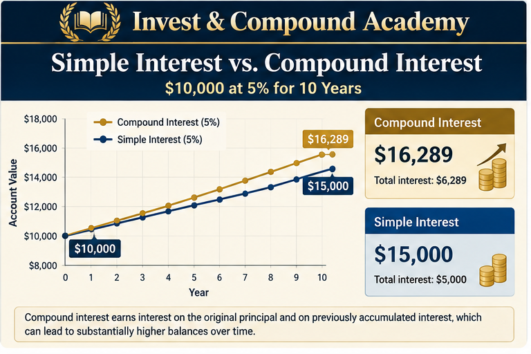
Simple interest is calculated only on the original principal. Compound interest is calculated on a balance that includes accumulated interest. Consider $10,000 earning 5% annually for ten years.
Simple Interest
Annual interest is: $10,000 × 5% = $500. Ten years produce $5,000 in total interest. The ending balance is $15,000.
Compound Interest
With annual compounding: $10,000 × 1.05^10 ≈ $16,288.95. The total interest is approximately $6,288.95. The difference between the two methods is approximately $1,288.95.
Why the Difference Expands
During the earliest years, the difference between simple and compound interest is relatively small. Over longer periods, the difference becomes larger because previously accumulated earnings generate further earnings. This is why time is such a powerful variable in the compounding equation. However, the example assumes a stable positive rate. Real-world investment results may fluctuate.
The compound balance exceeds the simple-interest balance because earlier interest stays in the interest-bearing base. It does not require a rising percentage rate. The two examples start with identical capital and exclude new deposits, so the difference can be attributed to the compounding convention.
Compound Interest Example: $1,000 at 5% for Ten Years
Consider an initial deposit of $1,000 earning 5% annually.
| Year | Ending balance |
|---|---|
| 0 | $1,000.00 |
| 1 | $1,050.00 |
| 2 | $1,102.50 |
| 3 | $1,157.63 |
| 4 | $1,215.51 |
| 5 | $1,276.28 |
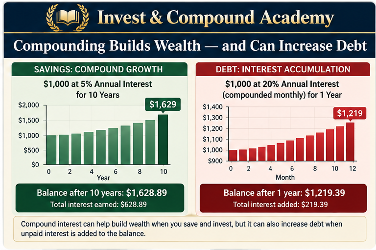
| 10 | $1,628.89 |
The balance increases by approximately $628.89 over ten years. The investor has not deposited any additional money. All growth comes from the assumed interest accumulation.
What Makes the Example Useful?
The example shows that the account grows even when the owner makes no new deposits. It also demonstrates that compound growth begins immediately. The additional interest may be modest at first, but it becomes progressively more meaningful as the balance increases.
What the Example Does Not Prove
The calculation does not demonstrate that every savings account will offer 5% for ten years. Deposit rates can change unless the account or instrument provides specific contractual terms. Taxes may also reduce the amount remaining to compound. For that reason, a mathematical example should not be confused with a savings product recommendation.
Compound Interest Example: $5,000 at 6% for Twenty Years
Now consider a larger starting amount and a longer period. Initial capital: $5,000. Assumed effective annual rate: 6%. Investment horizon: twenty years. The calculation produces approximately $16,035.68. The initial capital accounts for $5,000. The remaining approximately $11,035.68 represents accumulated growth.
Why the Dollar Gain Accelerates
A 6% return on the original $5,000 equals $300. A 6% return on a balance of $15,000 equals $900. The same percentage rate produces a much larger dollar increase because the balance has grown.
A Long-Term Perspective
The investment more than triples under the assumed conditions. However, the result depends on sustaining the specified growth rate. A market investment could generate a much higher or lower outcome. A fixed-income product may involve changing reinvestment rates after maturity. The key lesson is that the relationship between time and growth can be calculated precisely only after assumptions have been specified.
Compound Growth Example: $10,000 at 7% for Thirty Years
An extended investment horizon makes compounding particularly visible. Suppose an investor begins with $10,000. The portfolio generates a hypothetical constant 7% effective annual return. After thirty years: $10,000 × 1.07^30 ≈ $76,122.55. The hypothetical investment growth is approximately $66,122.55.
Why Thirty Years Produce More Than Three Times Ten-Year Growth
The future-value formula is exponential. The investment does not add the same dollar gain every decade. Each new period begins with the larger balance accumulated during the previous period.
The Role of Long-Term Equity Investing
Equity investors often seek to participate in the earnings growth and value creation of businesses over extended periods. However, stocks do not generate guaranteed annual interest. A constant 7% model is a planning assumption, not an actual sequence of stock-market returns. An investor may experience severe losses during the period. The realized compounded outcome will depend on those gains and losses.
Why the Starting Date Matters
Valuations, economic conditions, and future earnings influence actual returns. Two investors holding similar portfolios over different thirty-year periods may experience different outcomes. A projected value should therefore be considered one possible scenario within a wider range of uncertain results.
The Effect of Time: Fifteen Years vs. Thirty Years
Suppose two investors each deposit $25,000. Both use a hypothetical 8% effective annual growth assumption. Investor A leaves the money invested for fifteen years. Investor B leaves it invested for thirty years. After fifteen years, the projected balance is approximately $79,304. After thirty years, it is approximately $251,566. The longer horizon produces substantially greater wealth under the constant-rate assumption.
Why Time Cannot Always Be Replaced by Higher Returns
An investor who begins saving later may need larger contributions or higher growth to reach the same future balance. However, seeking higher returns often introduces greater uncertainty. The investor cannot simply choose a higher market return. Time and contribution capacity are generally more directly manageable than realized investment performance.
The Practical Lesson
Beginning earlier can expand the period available for reinvested returns to accumulate. But beginning later is not pointless. Contributions, realistic goals, and suitable asset allocation can still support financial progress. The relevant question is how to develop a feasible plan using the resources and time available.
Monthly Contributions: How Regular Savings Change Compounding
A one-time investment is only one model of wealth accumulation. Many investors build portfolios through regular contributions. These contributions increase principal while existing investments potentially continue generating returns.
A Combined Future-Value Formula
For an initial balance and fixed end-of-period contributions:
Here, P is the initial amount, C is the contribution per period, r is the effective return per period, and n is the number of periods. For a monthly contribution model based on an effective annual growth rate, the equivalent monthly rate is:
This conversion ensures that twelve periods compound to the stated effective annual rate.
Why Contribution Timing Matters
A contribution made at the beginning of a month has slightly more time to accumulate returns than one made at the end. The examples below assume end-of-month contributions. That convention should be displayed in any accompanying calculator.
For a zero growth rate, the annuity fraction is interpreted by its limit: FV = P + C × n. For example, $1,000 plus $50 for 240 months becomes $13,000 at zero growth. Dividing by a zero periodic return is unnecessary. The calculator handles this case directly.
Example: Starting With $1,000 and Adding $50 Monthly
Suppose an investor begins with $1,000. They add $50 at the end of each month for twenty years. Assume a constant 6% effective annual return. The projected final balance is approximately $25,879.07. The equivalent monthly return is approximately 0.486755%, not 0.50%.
The initial $1,000 grows to about $3,207.14; the stream of month-end deposits grows to about $22,671.94. Both components use the same monthly growth convention. Their unrounded sum produces the stated balance; adding rounded components can differ by a cent.
Total contributed capital is $13,000: the initial $1,000 plus $50 × 240 monthly deposits. Hypothetical investment growth is approximately $12,879.
Why This Is Different From Simple Saving
Without returns, the account would contain $13,000. Under the illustrative growth assumption, the balance approaches $25,900. Part of that difference comes from returns generated on earlier deposits. Those returns remain invested and can generate subsequent growth.
Why the Result Is Not Guaranteed
A diversified equity portfolio may experience negative returns in some years. A savings product may offer lower or changing interest rates. The model describes a constant-rate financial scenario, not a specific product’s expected outcome.
Example: Starting With $1,000 and Adding $100 Monthly
Now increase monthly contributions to $100 while keeping all other assumptions unchanged. Initial capital: $1,000. Monthly contribution: $100. Horizon: twenty years. Annual return assumption: 6%. The projected final balance is approximately $48,551. Total contributed capital equals $25,000. The hypothetical growth component is approximately $23,551.
What Changed?
The monthly contribution doubled. The investment return assumption did not change. The additional deposits increased the amount available to compound.
Why Contributions Are Powerful
Investors cannot control market returns. They have more direct influence over spending, saving, and contribution decisions, subject to income and financial obligations. Regular contributions can therefore provide a practical way to pursue long-term goals without relying on aggressive return assumptions.
Comparing Monthly Contribution Amounts
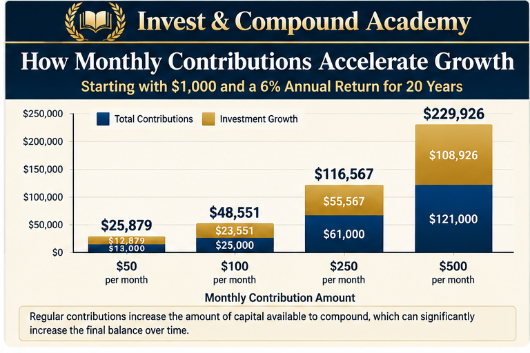
The following scenarios begin with $1,000, assume 6% effective annual growth, and continue for twenty years.
| Monthly contribution | Total contributed capital | Projected ending balance |
|---|---|---|
| $50 | $13,000 | $25,879 |
| $100 | $25,000 | $48,551 |
| $250 | $61,000 | $116,567 |
| $500 | $121,000 | $229,926 |
These are hypothetical values based on identical return assumptions. The table shows how contribution amounts influence long-term wealth. However, it should not be interpreted as encouragement to contribute more than a household can safely afford. Appropriate saving levels depend on essential expenses, financial obligations, emergency reserves, and available income.
The dollar-cost averaging pillar explains recurring purchases and average cost. Lump-sum investing versus DCA addresses a different decision: whether to invest an existing cash balance immediately or in stages. Money not yet earned cannot be invested earlier.
Why Contributions and Returns Must Be Reported Separately
A portfolio balance may increase for two very different reasons. First, the investor may deposit more capital. Second, the underlying investments may generate positive returns. A professional financial illustration should distinguish the two.
An Example
Suppose an investor starts with $10,000. Over several years, they contribute another $15,000. The ending balance reaches $32,000. The account increased by $22,000 relative to its initial value. But $15,000 of that increase came from additional deposits. The net investment growth is $7,000 before accounting for other relevant cash flows, costs, and adjustments.
Why Confusion Creates Misleading Claims
It would be inaccurate to describe the entire $22,000 increase as an investment return. Doing so overstates performance.
Time-Weighted and Money-Weighted Returns
Investors with irregular deposits and withdrawals may need more advanced performance measures. A time-weighted return attempts to isolate portfolio performance from external cash flows. A money-weighted return incorporates the timing and amounts of those flows. Both can be useful, but they answer different questions.
Our investment growth measurement guide explains the account reconciliation. In the example, $32,000 − $10,000 − $15,000 = $7,000 of dollar growth. That figure alone does not establish an annualized return; the dates of the contributions matter.
How Compounding Frequency Works
Compound interest can be calculated at different frequencies. Common conventions include annual, quarterly, monthly, and daily compounding. The effect depends on whether a quoted annual rate is nominal or effective.
Nominal Annual Rate
Suppose a deposit offers a nominal annual interest rate of 6% compounded monthly. The periodic rate is: 6% ÷ 12 = 0.5% per month. The effective annual rate is: (1 + 0.06/12)^12 − 1 ≈ 6.17%.
Effective Annual Rate
If a model specifies an effective annual rate of 6%, the equivalent monthly rate must be chosen so that twelve monthly periods produce exactly 6% growth. That rate is: 1.06^(1/12) − 1.
Why the Distinction Matters
Two calculators can produce different balances despite displaying the same numerical annual rate if they use different rate conventions. A trustworthy calculator must identify its assumptions clearly.
Daily Compounding
Some savings products calculate interest daily. The details depend on contractual terms, day-count methods, rate changes, and crediting schedules. Investors should consult the terms of the financial product rather than assume that daily compounding always produces a particular annual result.
For $10,000 at a 6% nominal annual rate compounded monthly, the year-end balance is $10,616.78. At a 6% effective annual rate, it is $10,600.00, regardless of an equivalent monthly modeling interval. Comparing the two without identifying the rate convention would attribute a rate difference to frequency alone.
Compounding Frequency Is Not the Same as Investment Performance
It is important to distinguish a contractual interest calculation from stock-market returns. A stock ETF does not necessarily credit a fixed interest percentage daily or monthly. The fund’s market value changes as underlying asset prices and distributions change. An annualized return can be converted into an equivalent monthly rate for mathematical modeling. That does not mean the actual fund will earn that monthly rate every month.
A Smooth Growth Model
A projection might assume 7% annual growth and use an equivalent monthly rate. The resulting line will appear smooth.
A Realistic Market Path
An actual equity portfolio might rise 15%, fall 20%, and subsequently recover. Its value may move unpredictably over short intervals.
Why This Matters for Investor Expectations
Smooth calculators are useful for understanding mathematical relationships. They are not substitutes for analyzing volatility, portfolio losses, liquidity, or the uncertainty of future investment outcomes.
How Investment Fees Compound Against Investors
Compounding can work against wealth accumulation when recurring costs reduce the invested balance. The U.S. Securities and Exchange Commission explains that fees reduce the amount of capital available to earn future returns. This creates a cumulative effect that becomes more meaningful over longer holding periods.
A Thirty-Year Example
Suppose an investor begins with $10,000. Assume a hypothetical gross annual return of 7%. Without recurring fees: $10,000 × 1.07^30 ≈ $76,123. Now assume an illustrative annual fee of 0.50%, charged multiplicatively against the year’s post-growth value. The annual factor becomes: 1.07 × 0.995. Over thirty years, the projected ending balance is approximately $65,495.
The difference is approximately $10,627.91. That gap includes fees deducted and the future growth those dollars no longer earn; it is not simply the sum of fee payments. The net effective annual growth rate in this convention is 6.465%, rather than exactly 6.50%. If the return entered in a calculator already reflects fund expenses, deducting those expenses again would double-count the cost.
Why Costs Matter Even When They Look Small
A half-percentage-point annual expense may appear insignificant. Over decades, it affects both the current account value and the capital available for future growth.
Why Fund Fees Are More Complex Than the Model
Actual ETF expenses generally accrue through fund assets over time. Transaction costs, portfolio tracking, securities lending, and other factors can also influence investor returns. The simplified calculation is educational, not an exact model of ETF expense accrual.
Comparing Similar Funds
Costs are particularly relevant when comparing funds providing substantially similar investment exposure. However, a lower fee does not automatically make a different, unsuitable investment strategy preferable. The asset allocation and investment objective must be considered first.
See the ETF research guide for assessing a fund’s mandate and costs, and the QQQ-to-QQQM switching analysis for the distinction between recurring savings and implementation costs. Compare funds with suitable, genuinely comparable exposures.
Inflation: Compounding Can Increase Prices Too
Inflation is often described as the gradual erosion of purchasing power. The same exponential mathematics that illustrates investment growth also describes sustained increases in the general price level.
A Price-Level Example
Suppose a basket of goods and services costs $10,000 today. Assume inflation averages 3% annually for twenty years. The future cost becomes: $10,000 × 1.03^20 ≈ $18,061. The purchasing power represented by $10,000 today would require approximately $18,061 in future nominal dollars.
Why Nominal Wealth Can Be Misleading
Suppose an investment grows at a hypothetical 7% annually for twenty years. The nominal balance increases from $10,000 to approximately $38,697. With 3% inflation over the same period, its value in today’s purchasing power is approximately $21,426. The nominal amount is much higher. But the real economic gain is smaller than the nominal growth alone suggests.
The Exact Real Return Formula
For 7% nominal growth and 3% inflation: 1.07 ÷ 1.03 − 1 ≈ 3.88%. The corresponding real compound growth rate is approximately 3.88% under the assumptions.
Why Investors Need Both Measures
Nominal returns describe the growth in currency units. Real returns describe purchasing-power growth. Both matter, but long-term financial goals ultimately relate to goods, services, and economic choices.
The inflation and investing pillar develops the purchasing-power question. Our recession guide examines declining economic activity, a separate concept. Neither a price-level assumption nor a recession label establishes a future portfolio return.
Compounding and Dividend Reinvestment
Some companies and ETFs distribute cash to shareholders. An investor may spend those distributions, retain them as cash, or use them to purchase additional investments. Dividend reinvestment can support accumulation because it increases the number of shares owned. However, distributions are not guaranteed investment growth.
A Simple Illustration
Suppose an investor owns 100 ETF shares priced at $50. The position has a market value of $5,000. The fund distributes $1 per share. The investor receives $100. If the distribution is reinvested at a share price of $49, ignoring fees and taxes, approximately 2.0408 additional shares could be purchased if fractional shares are supported.
The investor would then own approximately 102.0408 shares. Before reinvestment, the hypothetical position is worth $4,900 plus $100 cash. After reinvestment it remains worth $5,000, using full-precision shares and the assumed $49 price. The increase in share count is not an immediate investment gain. Rounding the share count for display should not be used to invent a loss of one cent.
Why the Share Price May Adjust
All else equal, the fund’s NAV adjusts downward by the distribution amount on the ex-distribution date. Market prices also reflect trading and other news; the actual quoted price need not fall by exactly that amount. A fund cannot distribute cash without that cash leaving its assets. The investor’s additional shares do not represent money created without economic cost.
What Reinvestment Actually Changes
Reinvestment keeps the distributed capital exposed to investment returns rather than converting it into cash held or spent. Future returns can then apply to the additional shares. But future returns may be positive or negative.
Why Yield Is Not Total Return
An ETF distributing 10% annually does not necessarily provide a 10% total return. Its share price may decline. Distributions may change. The fund may use strategies that sacrifice some upside. Investors should therefore evaluate total return and portfolio value alongside distribution rates.
The dividend yield versus total return guide explains why distributions should not be added again to an assumed total-return growth rate. What is dividend yield? explains the income ratio, while covered-call ETF financial reports examines portfolio operations, distributions and NAV.

Dividend Reinvestment With Whole Shares Only
Some brokerage accounts permit fractional dividend reinvestment. Others permit only whole-share purchases. This affects the speed and consistency with which distributions can be reinvested.
A Whole-Share Example
Suppose a fund pays a $75 distribution. Its shares trade at $40. A brokerage account permitting only whole shares may purchase one share for $40. The remaining $35 stays in cash, subject to the brokerage’s reinvestment rules. If the account does not support automatic reinvestment, the investor may need to place a manual purchase.
Why the Difference Matters
An investor planning long-term income reinvestment should not assume that every distribution will be fully deployed. Residual cash can accumulate. The difference may be modest for some portfolios and more important for smaller positions or higher-priced shares.
A Proper Calculator
A dividend reinvestment calculator should account for share prices, distribution amounts, reinvestment dates, purchase restrictions, and cash balances. Simply treating distribution yield as a guaranteed compound return would be misleading.
For a manual whole-share purchase, new shares = floor(available cash ÷ purchase price), before trading costs. Residual cash = available cash − purchase cost. Our whole-share ETF rebalancing workbook follows funded trades and rounding. Whether residual cash earns interest depends on the brokerage account.
Compounding and Bonds
Bonds can generate interest payments. However, bond compounding depends on what happens to those payments.
Coupon Payments
A conventional fixed-rate bond may pay coupons periodically. If an investor spends each coupon, the interest does not compound within the investment. If the coupons are reinvested, the investor may earn additional returns on them.
Reinvestment Risk
Future interest rates may differ from the bond’s original coupon rate. The investor cannot necessarily reinvest every payment at the same yield.
Bond Funds
A bond ETF holds a portfolio of securities whose prices change with yields, credit conditions, and other factors. The fund’s quoted yield is not automatically the rate at which the investor’s wealth will compound.
Why Yield and Return Differ
Yield measures a specified relationship among income, price, and cash flows. Total return also includes changes in market value. An investment may provide positive income while experiencing capital losses. For an accurate projection, the return measure must match the financial outcome being modeled.
Compounding Can Work Against Borrowers
Compound interest is not exclusively a wealth-building mechanism. It can also increase outstanding debt when unpaid interest is added to the balance and subsequently accrues interest. Credit cards and other borrowing arrangements may create substantial costs when balances are carried and interest accumulates.
A Simplified Debt Example
Suppose a borrower owes $1,000. Assume a nominal annual interest rate of 20%, compounded monthly. The borrower makes no payments, adds no new purchases, and incurs no other fees. After twelve months: $1,000 × (1 + 0.20/12)^12 ≈ $1,219.39. The balance increases by approximately $219.39.
Why Minimum Payments Matter
Actual credit-card terms are more complicated. Interest may be calculated using daily balances. Grace periods, payment allocation, penalties, fees, and minimum payment requirements differ. Nevertheless, the broader principle remains: carrying high-cost debt can undermine long-term wealth accumulation.
Debt Repayment vs. Investing
An investor considering additional market investments while carrying expensive debt should compare the interest costs specified by the debt agreement with the uncertain return on investments. Paying down debt can provide an economic benefit through reduced interest obligations. However, decisions should consider liquidity, contractual terms, taxes, and household circumstances.
Why a High Debt Rate Creates Serious Financial Pressure
A debt balance compounding at a high rate can grow rapidly if unpaid. The higher the rate, the faster interest accumulates. This is the same mathematical relationship that makes high investment growth assumptions appear attractive. But borrowers experience it in reverse.
Fixed Obligations
Debt payments can remain due even when employment income declines or investments lose value.
Compounding and Leverage
Borrowed capital used for investing creates additional risk. Investment losses can reduce the value of collateral while the debt remains outstanding.
Margin Accounts
Margin borrowing can generate interest expenses and introduce maintenance requirements. A decline in account equity may trigger forced liquidation under brokerage rules.
The Financial Planning Lesson
Understanding compounding should encourage attention to liabilities as well as assets. Growing investment wealth while allowing expensive debt to accumulate may produce disappointing net financial progress.
Borrowing risk interacts with market declines. Compare the market-correction pillar, correction versus bear market and bear-market mechanics. Correction durations and bear-market recovery times show why a lender’s repayment timetable cannot be assumed to match a market recovery.
The Rule of 72 and Compounding
The Rule of 72 offers a quick way to estimate the doubling time associated with a positive annual growth rate. The calculation is:
At 6% annual growth, the estimate is twelve years. At 8%, approximately nine years. The shortcut is especially useful for mental comparisons.
Why the Estimate Is Not Exact
The exact formula for a constant effective annual rate is:
At 8%, the exact result is approximately 9.01 years.
Why This Article Uses Full Future-Value Models
Doubling time answers one question. Many real-world financial objectives involve irregular contributions, different starting balances, withdrawals, or purchasing-power adjustments. Those situations require more complete formulas. The Rule of 72 is a useful companion to compound-growth models, not a replacement for them.
Our Rule of 72 calculator compares the shortcut with logarithmic doubling time. It is the better destination for sensitivity across doubling rates; these compound interest examples focus on the balances and cash flows behind the calculation.
How Volatility Changes Compounded Returns
An investment’s arithmetic average return can differ significantly from its compound growth rate. Consider a hypothetical investment that gains 40% one year and loses 30% the next. The arithmetic average is: (40% − 30%) ÷ 2 = 5%. However, the actual two-year growth factor is: 1.40 × 0.70 = 0.98. The portfolio loses 2% across the two years.
Why the Arithmetic Average Misleads
The arithmetic average adds percentage outcomes without accounting for how gains and losses affect the invested balance. Compound growth applies each return to the balance remaining after prior returns.
Understanding Volatility Drag
Large fluctuations can reduce compound growth relative to an arithmetic average. A loss reduces the capital base available to participate in subsequent gains.
Why Real Markets Are Different From Smooth Models
Actual equity returns vary. A steady 7% annual growth model does not imply that stocks rise 7% every year. Investors should understand that a projected compound annual return summarizes a possible long-term result under assumptions. It does not describe the guaranteed path to that result.
In this example, $10,000 becomes $14,000 and then $9,800. Its two-year CAGR is (0.98)^(1/2) − 1, approximately −1.01% per year. Reversing the same two returns produces $7,000 and then $9,800 if there are no cash flows. The path changes; the final product does not.
Why the Sequence of Returns Matters With Cash Flows
For a one-time fully invested balance with no external cash flows, changing the order of a fixed set of annual percentage returns does not change the mathematical product. However, the sequence becomes important when contributions or withdrawals occur.
Contributions During a Decline
An investor adding money after a substantial market decline may purchase more shares for the same contribution. If prices later recover, those shares can participate in the rebound.
Contributions Before a Decline
An investor purchasing immediately before a decline may experience losses on the newly contributed capital.
Withdrawals During a Decline
An investor withdrawing money while prices are depressed may need to sell more shares to obtain the required cash. Those shares are no longer available for subsequent recovery.
Retirement Implications
Sequence-of-returns risk is especially important when a portfolio funds regular spending. A high long-term arithmetic average does not guarantee that withdrawals will remain sustainable through an unfavorable return sequence. A retirement model should therefore go beyond constant annual growth.
A short contribution example makes the distinction visible. Start with $1,000, apply +20% then −20%, and add $100 after the first year: ($1,000 × 1.20 + $100) × 0.80 = $1,040. Reverse the returns: ($1,000 × 0.80 + $100) × 1.20 = $1,080. Both investors deposit $1,100, so both have a loss; the second loses $40 less. Without the intervening deposit, both finish at $960. Our compounding and withdrawals workbook examines spending cash flows.
Compound Interest and Retirement Planning
Retirement planning involves estimating future wealth and future spending. Both investment returns and inflation may compound over decades.
A Savings Example
Suppose an investor contributes a fixed amount each month to a suitable portfolio. The ending balance depends on contribution size, investment returns, fees, and the time available.
The Spending Side
Suppose current annual retirement spending would be $50,000. At a hypothetical constant 3% annual inflation rate for twenty-five years, an equivalent future spending level would exceed $100,000 annually.
Why Both Sides Matter
A portfolio may grow in nominal dollars while future spending requirements also rise. Retirement success depends on purchasing-power adequacy rather than nominal balance alone.
Withdrawal Strategies
Actual retirement outcomes depend on income sources, taxes, withdrawals, longevity, investment performance, and spending flexibility. A simplified future-value calculator is useful for accumulation planning. It is not a complete retirement sustainability model.
At 3% inflation, $50,000 × 1.03^25 is approximately $104,689. This is a future nominal annual spending amount with equivalent purchasing power, not an investment target or sustainable withdrawal recommendation. The $10,000 twenty-year projection separates nominal balances, deposits and real purchasing power.
How Compound Growth Works With ETFs
ETFs provide a convenient structure for holding portfolios of investments. Their growth potential depends on underlying assets, fees, distributions, and market returns.
Broad-Market Equity ETFs
These funds may hold large groups of companies. Over time, returns depend on business performance, valuations, and other market conditions.
Dividend ETFs
Dividend strategies may generate periodic income. However, distributions should be evaluated alongside changes in share value.
Bond ETFs
Bond funds generate returns through income and changes in market prices. Yield, duration, and credit quality influence outcomes.
Covered-Call ETFs
Covered-call strategies may distribute option-related income. But the strategy can limit upside and remains exposed to losses in underlying investments.
Why Structure Matters
The same compound-growth formula cannot establish equivalent expected results for every ETF. A projected return assumption must be considered in relation to the actual investment strategy and risk.
Start with the ETF beginner’s guide, ETF versus stock comparison and ETF versus mutual fund guide. ETF creation and redemption explains the wrapper. Portfolio construction and the maintenance workbook connect that structure to risk and ongoing decisions.
A dividend strategy such as the one discussed in our SCHD guide and the option-income approaches covered in our JEPI, JEPQ, SPYI and QQQI guides should not receive interchangeable return assumptions. Their mandates, distributions and risk exposures differ.
Compound Interest and Taxes
Taxes can reduce the amount of growth retained. The effect depends on jurisdiction, account type, and the nature of investment returns.
Taxable Interest
Interest earned in taxable accounts may create recurring tax obligations. If taxes are paid from investment earnings, less money remains available to compound.
Capital Gains
Taxes on realized capital gains may affect net investment outcomes. The timing of realization can matter.
Dividends and Distributions
Tax treatment varies across distribution types and jurisdictions. A dividend payment and a return-of-capital distribution may have different reporting consequences.
Registered and Tax-Advantaged Accounts
Certain retirement and savings accounts provide tax treatment intended to support financial objectives. However, rules differ between countries and accounts.
Why One Tax Formula Is Insufficient
A general compound interest calculator cannot accurately apply every investor’s tax circumstances through one universal rate. A high-quality tool should either model defined tax assumptions or state explicitly that taxes are excluded.
Common Compound Interest Mistakes
Assuming Compound Growth Is Guaranteed
Market investments can lose money. A mathematical projection does not establish a guaranteed return.
Confusing Simple and Compound Interest
Simple interest applies to the original principal. Compound interest includes accumulated interest in the interest-bearing balance.
Ignoring Contributions
A growing account balance may reflect new savings as well as investment gains.
Using Arithmetic Average Returns
An arithmetic average may not describe the compound rate actually achieved.
Ignoring Inflation
Nominal wealth growth does not necessarily indicate equivalent purchasing-power growth.
Ignoring Fees
Recurring costs can materially reduce long-term returns.
Treating Distribution Yield as Total Return
High cash distributions do not guarantee compounding at an equivalent rate.
Ignoring Debt Compounding
High borrowing costs can undermine progress toward financial goals.
Mixing Annual Rate Conventions
Nominal and effective annual rates are not identical when interest compounds more than once per year.
Ignoring Taxes
Actual after-tax balances can differ from gross projections.
Assuming More Frequent Compounding Guarantees Better Investments
Compounding frequency is only one characteristic of a product. Risk, costs, and underlying returns remain important.
Overestimating Future Returns
A high projected balance does not prove that the assumed return is achievable.
Use what to do during a correction and buying during a correction for decision frameworks. Historical corrections, warning signs, correction frequency and correction statistics provide market context. They do not turn a constant-rate worksheet into a forecast.
Frequently Asked Questions
What Is Compound Interest in Simple Terms?
Compound interest means earning interest on an amount that includes previously accumulated interest.
Can You Give a Simple Example?
A $1,000 account earning 5% annually grows to $1,050 after one year and $1,102.50 after two years, assuming interest remains in the account.
What Is the Compound Interest Formula?
For annual compounding, future value equals principal multiplied by one plus the annual rate raised to the number of years.
What Is the Difference Between Simple and Compound Interest?
Simple interest is calculated on original principal. Compound interest also applies to accumulated interest.
How Much Does $1,000 Grow at 5% for Ten Years?
Approximately $1,628.89 with constant annual compounding and no additional deposits.
How Much Does $5,000 Grow at 6% for Twenty Years?
Approximately $16,035.68 under the stated constant-rate assumption.
Can Compound Interest Make Someone Wealthy?
Compounding can contribute significantly to wealth accumulation, but results depend on capital, contributions, actual returns, time, and financial risks.
Is Compounding Guaranteed in the Stock Market?
No. Equity returns are uncertain and can be negative.
How Do Monthly Contributions Affect Compounding?
They increase principal over time, allowing new deposits and any retained earnings to participate in subsequent investment returns.
Does Monthly Compounding Beat Annual Compounding?
Under certain nominal-rate conventions, more frequent compounding can produce a higher effective rate. Results depend on the quoted terms.
Is Dividend Reinvestment the Same as Compound Interest?
Dividend reinvestment can contribute to compounded investment returns, but dividends and share-price movements are not guaranteed interest.
Do ETFs Compound Automatically?
ETF total returns can compound when gains remain invested, but outcomes depend on underlying performance, distributions, and reinvestment decisions.
Does a 10% Dividend Yield Mean 10% Annual Growth?
No. Distribution yield and total return are different measurements.
How Does Inflation Affect Compounding?
Inflation increases the general price level and reduces the purchasing power of future nominal balances.
How Do Fees Affect Compound Growth?
Fees reduce the capital available to earn future returns, potentially creating substantial long-term differences.
Can Debt Compound?
Yes. Under applicable contract terms, unpaid interest may accumulate and generate further interest.
Is Paying Off Debt Better Than Investing?
The appropriate decision depends on debt costs, investment risks, liquidity, taxes, and financial circumstances.
What Is the Rule of 72?
It is a shortcut that estimates doubling time by dividing 72 by a positive annual percentage growth rate.
Why Does Starting Earlier Matter?
Starting earlier can provide more time for returns to accumulate and generate subsequent returns.
What Is the Biggest Limitation of Compound Interest Calculators?
They rely on assumptions about returns, timing, and costs that may not match actual future outcomes.
What These Compound Interest Examples Show
Compound interest is one of the most useful concepts in financial education because it explains how accumulated earnings can generate further earnings. A relatively small balance can become much larger when positive returns are retained over an extended period. Regular contributions can increase the amount available for investment, while time allows earlier deposits to participate in subsequent growth. However, the mathematics should not obscure the financial reality. Investment returns are uncertain. Stocks and ETFs can experience severe declines. A projected growth rate does not establish that a future portfolio balance will be achieved.
Fees, taxes, withdrawals, and inflation can reduce the value of the eventual result. Debt can also compound, increasing financial obligations rather than building wealth. For that reason, compounding should be understood in the context of both assets and liabilities. A sound financial strategy considers how savings accumulate, how investments generate returns, how expenses reduce those returns, and how purchasing power changes over time. It also distinguishes new contributions from genuine investment performance. The most important variables are not always those investors can control.
Future market returns remain uncertain, but contribution habits, cost awareness, diversification, debt management, and financial planning processes can often be managed more directly. Compound interest is valuable because it rewards the accumulation and retention of earnings under favorable conditions. It is not a substitute for careful asset selection, appropriate risk exposure, or realistic expectations.
Explore the Earlier Academy Pillars
Connect these worked examples with the eighteen earlier pillars on market behavior, economic conditions, investment methods and growth mathematics.
Continue Learning in the Invest & Compound Academy
Follow the question that matters for your next calculation: doubling time, future value, recurring purchases, deployment, purchasing power or distributions.
Compound interest examples, reinvestment and savings mathematics
Market Correction Pillar | Indexes and Markets | Portfolio Construction
Sources and Further Reading
Reference review: October 19, 2026. Official education sources support the concepts of compounding, expenses and purchasing power. All balances, hypothetical growth paths, distribution scenarios and debt illustrations are mathematical examples, not historical performance claims or quoted product terms. Calculations retain full precision before display rounding.
- Consumer Financial Protection Bureau: How Does Compound Interest Work? General explanation of accumulated interest; last reviewed October 19, 2023.
- SEC Investor.gov: Compound Interest Calculator — initial investment, contributions, periods, rates and frequency.
- SEC Investor.gov: How Fees and Expenses Affect Your Investment Portfolio — Investor Bulletin, July 23, 2025.
- U.S. Bureau of Labor Statistics: Purchasing Power and Constant Dollars — comparing nominal values and purchasing power.
This article provides general financial education, not personalized financial, investment, tax or legal advice or a recommendation to buy, sell or hold a security.
Constant growth rates and simplified fees demonstrate mathematical relationships. Actual returns fluctuate, can be negative and may involve permanent loss of capital. Compounding does not remove investment risk.
Taxes, fees, inflation, distributions, cash flows and borrowing terms affect outcomes. Calculators do not forecast returns or reproduce every deposit or loan agreement. Read the applicable terms and consider your circumstances before making financial decisions.